Introduction
As we mentioned before, Drive Test is important for a more complete analysis of the network. The various post-processing tools available have a complete set for this analysis, but sometimes our work can be much simplified, and why not, sometimes getting a better result.
This is particularly the case for the custom processing of drive test - we can not even have the power of algorithms and details of some software, but we got results surprisingly simple and efficient. Today we’ll learn a creative way to plot the data signal level of a network in Google Earth, no matter what has been the equipment / software that has made the collection of the drive test.
Purpose
From the data collected in a drive test, generate an output file in Google Earth KML format with the information plotted according to our choices.
In other words, plot the data from the drive test on Google Earth, much as we do with thematic maps in MapInfo.
Our audience is from students to experienced professionals. Therefore we ask for a little understanding and tolerance if some some of the concepts presented today are too basic for you. Moreover, all the tutorials, codes and programs are at a continuous process of editing. This means that if we find any error, for example, grammar or spelling, try to fix it as soon as possible. We would also like to receive your feedback, informing us of errors or passages that were confusing and deserve to be rewritten.
File Structure
Another new module. As always, we will increase our structure to suit the needs. You’ve probably noticed how the organization is important. Every time the tool Hunter grows, it becomes more important to keep the interconnected modules.
This is a module that also uses Google Earth - GE - so the structure is created below the folder GE. Create the directory DriveTest (1) as the main directory of this module. The other directories Data (2) Output (3) and Scripts (4) are the standard modules of our tool. Just remembering, are respectively the directories where are our incoming data files collected in the drive test, the output data, where today a file. KML with the formatted data, and directory scripts, now with the file that does the processing, and we will create from now.
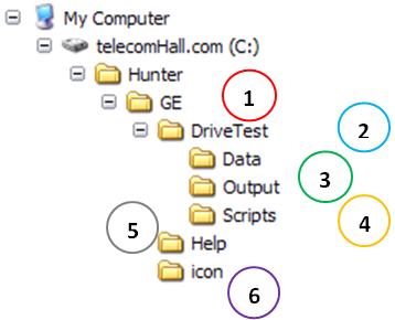
Note that we have a directory of Help - Help (5). In this directory store all the auxiliary file for that module specifically. Also note that this module uses the directory icon (6), remembering that this directory had been created earlier, since it is shared with several modules.
Input data
Our main goal is to create an application that is compatible with the output of whatever equipment or software that has been used to perform the drive test.
Each software has a specific output format, and would be very complicated now - although not impossible - to create an application that reads data directly exported.
Fortunately, all such software has the facility to export to most common file as TXT, CSV or XML.
This is the simplest, and for several reasons, we use the principle. In future, if there is interest, we can go deeper and show how to handle the data directly in the proprietary format of each software. We emphasize that this is not only simple, so let’s not talk about this today.
Note: see, this is not necessarily a problem. For example, if you want to analyze their data in Mapinfo, first you must also export the data to a format of MapInfo. Moreover, in the case of our custom tool, is not to do anything else besides exporting the data from drive test software.
So we can have our input as text (.TXT or .CSV) or as Excel spreadsheets (.XLS or .XLSX). These formats are currently supported by our tool customized GE Hunter Drive Test. See who is already very flexible, since there is a collection of software that do not export to at least one of these formats.
How this module works
The steps below show how a simplified procedure for obtaining the final files.
-
- Perform data collection, using any device or software collection,
-
- Export the data collected for TXT, CSV, XLS or XLSX, and store one or more files in the folder C:\Hunter\GE\DriveTest\Data;
-
- Open the file GE_DriveTest_1.0_RUN.mdb located in the Scripts folder, run the macro GE_DriveTest_Main_RUN and wait for processing;
- The script checks if there is any file in the format above, and if found, it is the same for a table DriveTest, then creates the output file, based on information from consultation qry_DriveTest. This query has a few tricks and devices, as discussed below.
Pronto. The data is already available in the Output folder C:\Hunter\GE\DriveTest\Output.
Input Data
To demonstrate, let’s follow the above procedure, showing how the data are processed. You must remember that we just use dummy data in our examples, and that in a previous tutorial we already export dummy data to test our network drive for file log_exported. So let’s use that same file today.
Importing a text file into Access
Once one or more files are in the Data directory, you can run the macro, and generate a KML file corresponding to each of them.
And how is this done? Well, manually importing data into Access has already been shown in a previous tutorial. Let’s see how this is done via VBA code.
To import a file in an automated fashion, we must first have an Import Specification. What does this mean? Simply put, is a specification that tells Access how the format of the text file it is importing. For example if the file uses a comma or tab as separator, if the first line has the name of the fields, etc… So the first thing to do is create our import specification to a text file with our format.
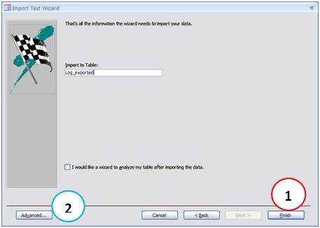
To do this, import the file manually through the interface normal Access Menu - External Data -> Text File. But in the last step, do NOT click Finish (1). Instead, click the Advanced button (2).
Note that getting there is stored information that Access will use to complete the import. Since we want to use this specification other times, we save this specification by clicking on Save As … (1).
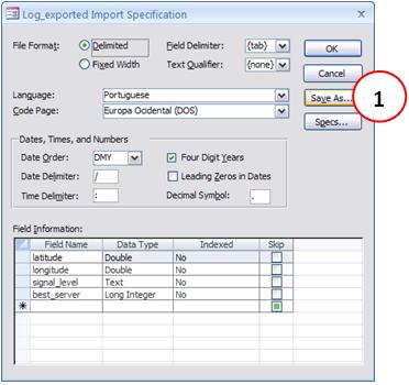
And save this specification as DriveTest Import Specification (1). Click the OK button (2).
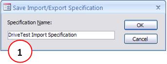
We don’t have to finish importation, we already did what we wanted, which was to save the specification of this file.
Note: If you complete the import, Access will ask if you still want to save all these steps to import. Do not mistake, this is something else, and we will not need it, we have saved the specification, which is what interests us. Simply click Close.
Pronto. What we have so far? Access already know what are the characteristics of our archive. Now whenever we need to import it again - either with new data, but in this format - we can use this specification.
And we’ll do it directly in code.
The command that does this is the TransferText.
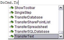
And the arguments are very intuitive:
![]()
-
TransferType: where we say it is an import delimited or fixed length columns. In our case it is tab delimited, choose acImportDelimited.
-
SpecificationName: the name of the import specification that saved previously in the case DriveTest Import Specification.
-
tablename: the table name to which we will import the file, if DriveTest.
-
FileName: full name of the file, with the path. In our case, C:\Hunter\GE\DriveTest\Data\Hunter_GE_DriveTest.txt.
-
HasFieldNames: the first line of our file has the name of the fields, so we put Yes
-
HTMLTableName: can leave blank.
-
CodePage: can leave blank.
And our code responsible for import:
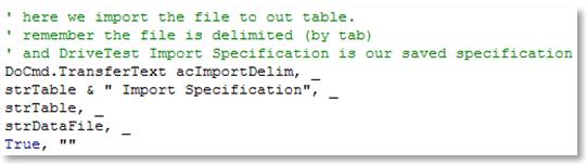
Note: Note that we use the sign _ at the end of the line, indicating that it is not over. This is only meant for human reading, lest they be huge lines, and it becomes easier to analyze the code.
Sure, when that line is executed, the file C:\Hunter\GE\DriveTest\Data\Hunter_GE_DriveTest.txt will be imported into the table DriveTest, with the fields defined in accordance with the import specification DriveTest Import Specification, as previously saved.
Now we can use this data and write the KML file.
Handling data
But before we write the KML file, we need to do some treatments, because the data are not in the best possible way. And for that we will use consultations.
In this tutorial, we will have the following flowchart:
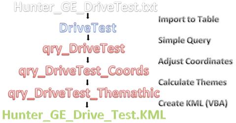
Following the flowchart, we already imported the file Hunter_GE_DriveTest.txt into the table DriveTest.
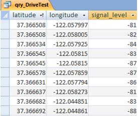
Now we create a simple query, only to look up the data from DriveTest base table. As mentioned earlier, it is never good to use queries directly to our table bases. This query works something like a bridge. Trying to explain, the first query, which is more or less as a mirror of the table (and for that reason perhaps you think that it did not matter at all), but allows us to make some adjustments, such as changing some kind of data - such as text to integer. But okay, maybe now is still a little early for you to understand. Anyway, let’s continue from the consultation qry_DriveTest, a mirror of our table.
See the query result qry_DriveTest.
The next step is interesting and requires a brief explanation of how the collection is performed.
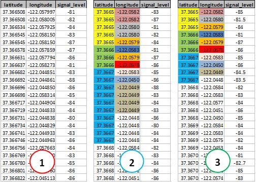
The drive test equipment using GPS, and collect data continuously. And sometimes it happens that at some points are taken several measures. Or at least in very close to each other. All right, we could plot all the points raised, but had a small problem, especially when the drive test is very large: more points than necessary to represent the delay to load. So we use the device to limit the points in the fourth decimal latitude and longitude. Then, we grouped these new sets of points, making the necessary operations in other fields. For example, to the signal level, we take the average.
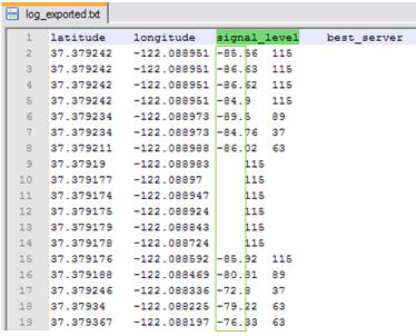
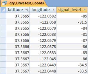
The following tables help us better understand the device used. In the first table (1) we have the data as exported in the case with 6 decimal places. The second table (2) presents data from the same table, only now with latitude and longitude to four decimal places, and equal values grouped by color. At the last table (3) we have the query result qyr_DriveTest_Coords, used in plotting the data. Note that new pair of latitude and longitude are grouped, and the new signal_level field contains the average signal in points grouped.
This approach proves to be much closer to reality. Also because thus we increased the precision at each point, it is as if we had performed several measurements and we used the average. Simple and efficient, no?
Two important information: you can choose another type of approach, such as 5 decimal places, or even not use that approach - whether to have a very great detail, all points - just make changes in this consultation. Another thing: do not worry if you do not understand. Over time, this will become clearer to you.
See now the query result qry_DriveTest_Coords.
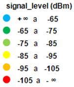
Continuing, we reached the point where we must create the themes for our records. That is, each record will have a new field, calculated according to the data we wish to create the thematic map. For example, if the signal level is between -75 and -65 dBm, and yellow coloring, if you are between -85 and -75 dBm, as gray color, and so on.
So we created the field themathic_signal_level calculated with the formula shown below.
themathic_signal_level :
IIf(([signal_level]<-105),“red”,
IIf(([signal_level]>=-105 And [signal_level]<-95),“orange”,
IIf(([signal_level]>=-95 And [signal_level]<-85),“yellow”,
IIf(([signal_level]>=-85 And [signal_level]<-75),“lightgreen”,
IIf(([signal_level]>=-75 And [signal_level]<-65),“green”,
IIf(([signal_level]>=-65),“blue”,
“”))))))
Notice how our data are now. In the new query qry_DriveTest_Themathic, we themathic_signal_level field. It is based on the values of this field that assign styles to each point (marker) on Google Earth.
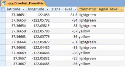
Note that for each indicator that we create, we have a different legend. Below is the caption for signal_level. The auxiliary files with these legends in wrod are found in the Help directory of the module GE. In the future we will see a little more about creating captions and indicators.
Okay, now we can write the KML file, using data from this query. So we’ll continue …
The Code
All artifacts and particularities that the tool uses to plot the data have already been mentioned above, and you can already adapt their code to function this way. If you subscribe, please remember that the simplest way to learn the code is read it, since it is fully reviewed. Any questions, please contact our support.
The following is an initial part of the code, where the most important points have already been expounded in this or previous tutorial.
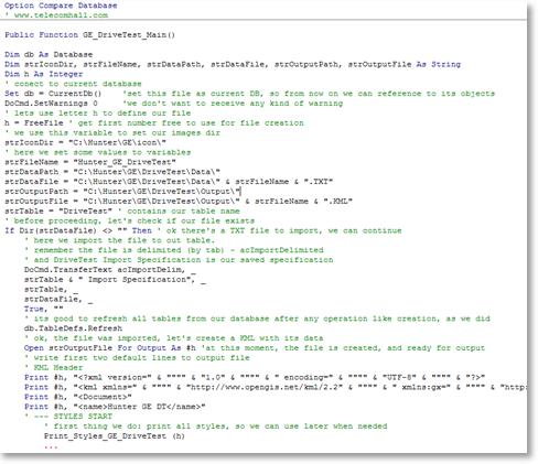
Important: remember that our intention is above all to teach. You will notice that some parts of original code are simplified. For example, the code imports a fixed file, or hard-coded - even if that name is coming from a variable strFileName. If we change the file name to something other than Hunter_GE_DriveTest.txt will no longer work.
This is not an ideal behavior, and certainly not what we use. But we must move slowly, there are several other items and features that will be added to that module and exeplicadas GE DriveTest.
We’ll still have further improvements in generic form, as form creation - interfaces - to facilitate interaction. Again, this is being gradually established, so that you perceive.
Returning to our application today, although in some ways quite simple especially for those who already program, the result is quite interesting, as shown below.
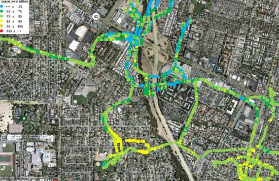
Note: It is important that you know that the data are not perfectly aligned with the streets of Google Earth because they were generated randomly and not by an error in our program. When you use with real data from your network, you will see that the data are perfectly aligned, except for some inaccuracies of GPS.
Note that all points are clickable, both in the main interface, the browser on the side. For example, if you wish to navigate to a specific signal level bad, just double click on it.
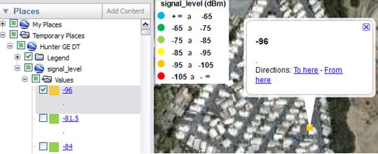
Furthermore, you use all the resources that are available. For example, you can open our network Hunter_GE_Network, and analyzing drive test along with the information sector. You can quickly verify that the antenna is being used, what the tilde, etc…
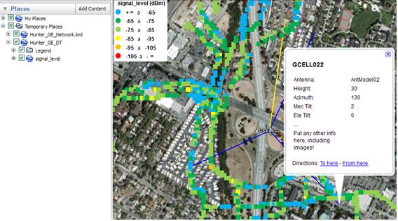
All of this information, together with others that we will see, provide an analysis much more quickly and efficiently. That’s our goal: to create a single, centralized, and all available key information needed to take action.
Soon you will see how this set of information is important and essential in everyday life of a professional in the field of Telecom and IT.
Conclusion
We learned today how to plot data from a drive test in Google Earth, from a simple text file, exported by the software collection / processing.
In terms of programming, we saw how it’s done importing a text file by VBA code. While the import has not been dynamic - we import a file with fixed name and format, used to understand the needs of future implementations that minimize this limitation.
The end result, although simple, allows us to see the importance of tools that help us both in processing speed, accuracy in analysis and ease of operation. This is the main objective of the Hunter system, which gradually you will know.
We hope you’ve enjoyed. If you have any doubts, find the answers posting your comments in the blog or via our support via chat or email.
Till our next meeting, and remember: Your success is our success!
Download
Download Source Code: Blog_013_Hunter_GE_DriveTest_(signal_level).zip (1.5 MB)