Introduction
The efficiency of a cellular network depends of its correct configuration and adjustment of radiant systems: their transmit and receive antennas.
And one of the more important system optimizations task is based on correct adjusting tilts, or the inclination of the antenna in relation to an axis. With the tilt, we direct irradiation further down (or higher), concentrating the energy in the new desired direction.
When the antenna is tilted down, we call it ‘downtilt’, which is the most common use. If the inclination is up (very rare and extreme cases), we call ‘uptilt’.
Note: for this reason, when we refer to tilt in this tutorial this means we’re talking about ‘downtilt’. When we need to talk about ‘uptilt’ we’ll use this nomenclature, explicitly.
The tilt is used when we want to reduce interference and/or coverage in some specific areas, having each cell to meet only its designed area.
Although this is a complex issue, let’s try to understand in a simple way how all of this works?
But Before: Antenna Radiation Diagram
Before we talk about tilt, it is necessary to talk about another very important concept: the antennas radiation diagram.
The antenna irradiation diagram is a graphical representation of how the signal is spread through that antenna, in all directions.
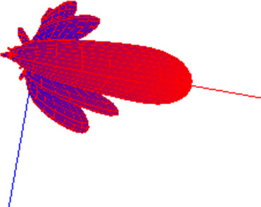
It is easier to understand by seeing an example of a 3D diagram of an antenna (in this case, a directional antenna with horizontal beamwidth of 65 degrees).
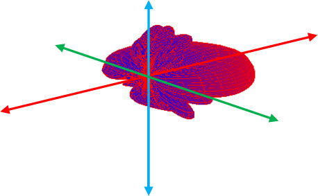
The representation shows, in a simplified form, the gain of the signal on each of these directions. From the center point of the X, Y and Z axis, we have the gain in all directions.
If you look at the diagram of antenna ‘from above’, and also ‘aside’, we would see something like the one shown below.
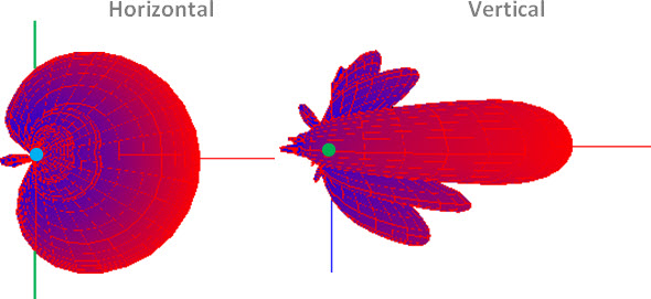
These are the Horizontal (viewed from above) and Vertical (viewed from the side) diagrams of the antenna.
But while this visualization is good to understand the subject, in practice do not work with the 3D diagrams, but with the 2D representation.
So, the same antenna we have above may be represented as follows.
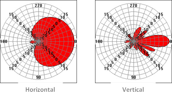
Usually the diagrams have rows and numbers to help us verify the exact ‘behavior’ in each of the directions.
- The ‘straight lines’ tells us the direction (azimuth) – as the numbers 0, 90, 180 and 270 in the figures above.
- And the ‘curves’ or ‘circles’ tells us the gain in that direction (for example, the larger circle tells you where the antenna achieves a gain of 15 db).
According to the applied tilt, we’ll have a different modified diagram, i.e. we affect the coverage area. For example, if we apply an electrical tilt of 10 degrees to antenna shown above, its diagrams are as shown below.
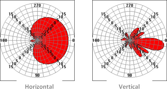
The most important here is to understand this ‘concept’, and be able to imagine how would the 3D model be, a combination of its Horizontal and Vertical diagrams.
Now yes: what is Tilt?
Right, now we can talk specifically about Tilt. Let’s start reminding what is the Tilt of an antenna, and what is its purpose.
The tilt represents the inclination or angle of the antenna to its axis.
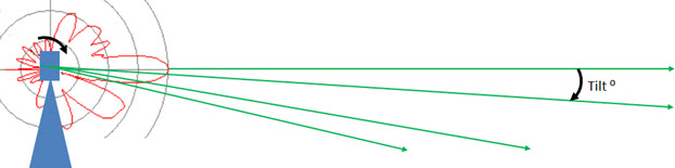
As we have seen, when we apply a tilt, we change the antenna radiation diagram.
For a standard antenna, without Tilt, the diagram is formed as we see in the following figure.
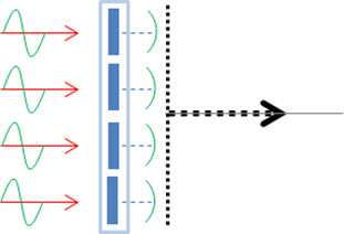
There are two possible types of Tilt (which can be applied together): the electrical Tilt and Mechanical Tilt.
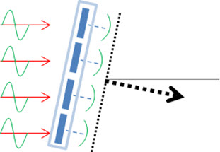
The mechanical tilt is very easy to be understood: tilting the antenna, through specific accessories on its bracket, without changing the phase of the input signal, the diagram (and consequently the signal propagation directions) is modified.
And for the electrical tilt, the modification of the diagram is obtained by changing the characteristics of signal phase of each element of the antenna, as seen below.
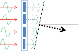
Note : the electrical tilt can have a fixed value, or can be variable, usually adjusted through an accessory such as a rod or bolt with markings. This adjustment can be either manual or remote, in the latter case being known as ‘RET’ (Remote Electrical Tilt) – usually a small engine connected to the screw stem/regulator that does the job of adjusting the tilt.
With no doubt the best option is to use antennas with variable electrical tilt AND remote adjustment possibility, because it gives much more flexibility and ease to the optimizer.
However these solutions are usually more expensive, and therefore the antennas with manual variable electrical tilt option are more common.
So, if you don’t have the budget for antennas with RET, choose at least antennas with manual but ‘variable’ electrical tilt – only when you have no choice/options, choose antennas with fixed electrical tilt.
Changes in Radiation diagrams: depends on the Tilt Type
We have already seen that when we apply a tilt (electrical or mechanical) to an antenna, we have change of signal propagation, because we change the 3D diagram as discussed earlier.
But this variation is also different depending on the type of electrical or mechanical tilt. Therefore, it is very important to understand how the irradiated signal is affected in each case.
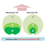
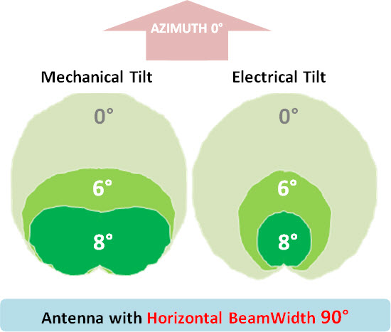
To explain these effects through calculations and definitions of db, null and gains on the diagram is possible. But the following figures shows it in a a much more simplified way, as horizontal beamwidth behaves when we apply electrical and mechanical tilt to an antenna.
See how is the Horizontal Irradiation Diagram for an antenna with horizontal beamwidth of 90 degrees.
Of course, depending on the horizontal beamwidth, we’ll have other figures. But the idea, or the ‘behavior’ is the same. Below, we have the same result for an antenna with horizontal beamwidth of 65 degrees.
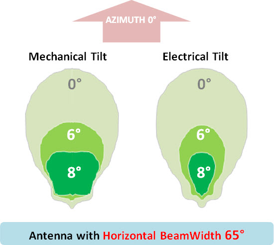
Our goal it that with the pictures above you can understand how each type of tilt affects the end result in coverage – one of the most important goals of this tutorial.
But the best way to verify this concept in practice is by checking the final coverage that each one produces.
To do this, then let’s take as a reference a simple ‘coverage prediction’ of a sample cell. (These results could also be obtained from detailed Drive Test measurements in the cell region).
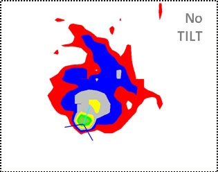
Then we will generate 2 more predictions: the first with electrical tilt = 8 degrees (and no mechanical tilt). And the second with only mechanical of 8 degrees.
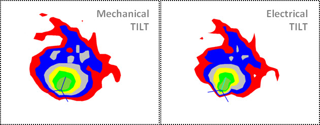
Analyzing the diagrams for both types of tilt, as well as the results of the predictions (these results also can also be proven by drive test measures) we find that:
With the mechanical tilt, the coverage area is reduced in central direction, but the coverage area in side directions are increased.
With the electrical tilt, the coverage area suffers a uniform reduction in the direction of the antenna azimuth, that is, the gain is reduced uniformly.
Conclusion: the advantages of one tilt type to another tilt type are very based on its application – when one of the above two result is desired/required.
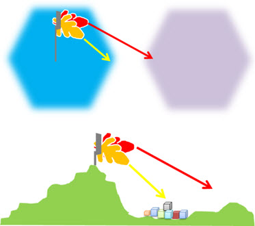
But in General, the basic concept of tilt is that when we apply the tilt to an antenna, we improve the signal in areas close to the site, and reduced the coverage in more remote locations. In other words, when we’re adjusting the tilt we seek a signal as strong as possible in areas of interest (where the traffic must be), and similarly, a signal the weakest as possible beyond the borders of the cell.
Of course everything depends on the ‘variables’ involved as tilt angle, height and type of antenna and also of topography and existing obstacles.
Roughly, but that can be used in practice, the tilt angles can be estimated through simple calculation of the vertical angle between the antenna and the area of interest.
In other words, we chose a tilt angle in such a way that the desired coverage areas are in the direction of vertical diagram.
It is important to compare:
- the antenna angle toward the area of interest;
- the antenna vertical diagram.
We must also take into account the antenna nulls. These null points in antenna diagrams should not be targeted to important areas.
As basic formula, we have:
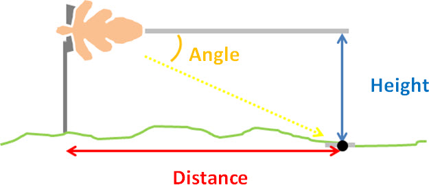
Angle = ArcTAN (Height / Distance)
Note: the height and distance must be in the same measurement units.
Recommendations
The main recommendation to be followed when applying tilts, is to use it with caution. Although the tilt can reduce interference, it can also reduce coverage, especially in indoor locations.
So, calculations (and measurements) must be made to predict (and check) the results, and if that means coverage loss, we should re-evaluate the tilt.
It is a good practice to define some ‘same’ typical values (default) of tilt to be applied on the network cells, varying only based on region, cell size, and antennas heights and types.
It is recommended not to use too aggressive values: it is better to start with a small tilt in all cells, and then go making any adjustments as needed to improve coverage/interference.
When using mechanical tilt, remember that the horizontal beamwidth is wider to the antenna sides, which can represent a problem in C/I ratio in the coverage of neighboring cells.
Always make a local verification, after changing any tilt, by less than it has been. This means assessing the coverage and quality in the area of the changed cell, and also in the affected region. Always remember that a problem may have been solved … but another may have arisen!
Documentation
The documentation is a very important task in all activities of the telecommunications area. But this importance is even greater when we talk about Radiant System documentation (including tilts).
It is very important to know exactly ‘what’ we have currently configured at each network cell. And equally important, to know ‘why’ that given value has changed, or optimized.
Professionals who do not follow this rule often must perform rework for several reasons – simply because the changes were not properly documented.
For example, if a particular tilt was applied to remove the interfering signal at a VIP customer, the same should go back to the original value when the frequency plan is fixed.
Other case for example is if the tilt was applied due to problems of congestion. After the sector expansion (TRX, Carriers, etc…), the tilt must return to the previous value, reaching a greater coverage area, and consequently, generating overall greater revenue.
Another case still is when we have the activation of a new site: all neighboring sites should be reevaluated – both tilts and azimutes.
Of course that each case should be evaluated according to its characteristics – and only then deciding to aplly final tilt values. For example, if there is a large building in front of an antenna, increasing the tilt could end up completely eliminating the signal.
In all cases, common sense should prevail, evaluating the result through all the possible tools and calculations (as Predictions), data collection (as Drive Test) and KPI’s.
Practical Values
As we can see, there’s not a ‘rule’, or default value for all the tilts of a network.
But considering the most values found in field, reasonable values are:
- 15 dBi gain: default tilt between 7 and 8 degrees (being 8 degrees to smaller cells).
- 18 dBi gain: default tilt between 3.5 and 4 degrees (again, being 4 degrees to smaller cells).
These values have tipically 3 to 5 dB of loss on the horizon.
Note: the default tilt is slightly larger in smaller cells because these are cells are in dense areas, and a slightly smaller coverage loss won’t have as much effect as in larger cells. And in cases of very small cells, the tilt is practically mandatory – otherwise we run the risk of creating very poor coverage areas on its edges due to antenna nulls.
It is easier to control a network when all cells have approximately the same value on almost all antennas: with a small value or even without tilt applied to all cells, we have an almost negligible coverage loss, and a good C/I level.
Thus, we can worry about - and focus - only on the more problematic cells.
When you apply tilts in antennas, make in a structured manner, for example with steps of 2 or 3 degrees – document it and also let your team know this steps.
As already mentioned, the mechanical tilt is often changed through the adjust of mechanical devices (1) and (2) that fixes the antennas to brackets.
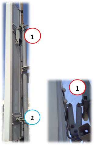
And the electrical tilt can be modified for example through rods or screws, usually located at the bottom of the antenna, which when moved, applies some corresponding tilt to the antenna.
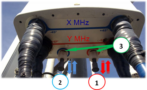
For example in the above figure, we have a dual antenna (two frequency bands), and of course, 2 rods (1) and (2) that are moved around, and have a small display (3) indicating the corresponding electrical tilt – one for each band.
And what are the applications?
In the definitions so far, we’ve already seen that the tilts applications are several, as to minimize neighboring cells unwanted overlap, e.g. improving the conditions for the handover. Also we can apply tilt to remove local interference and increase the traffic capacity, and also cases where we simply want to change the size of certain cells, for example when we insert a new cell.
In A Nutshell : the most important thing is to understand the concept, or effect of each type of tilt, so that you can apply it as best as possible in each situation.
Final Tips
The tilt subject is far more comprehensive that we (tried to) demonstrate here today, but we believe it is enough for you to understand the basic concepts.
A final tip is when applying tilts in antennas with more than one band.
This is because in different frequency bands, we have different propagation losses. For this reason, antennae that allow more than one band has different propagation diagrams, and above all, different gains and electrical tilt range.
And what’s the problem?
Well, suppose as an example an antenna that has the band X, the lower, and a band Y, highest.
Analyzing the characteristics of this specific antenna, you’ll see that the ranges of electrical tilt are different for each band.
For example, for this same dual antenna we can have:
- X band: electrical tilt range from 0 to 10 degrees.
- Y band: electrical tilt range from 0 to 6 degrees.
The gain of the lower band is always smaller, like to ‘adjust’ the smaller loss that this band has in relation to each other. In this way, we can achieve a coverage area roughly equal on both bands – of course if we use ‘equivalent’ tilts.
Okay, but in the example above, the maximum is 10 and 6. What would be equivalent tilt?
So the tip is this: always pay attention to the correlation of tilts between antennas with more than one band being transmitted!
The suggestion is to maintain an auxiliary table, with the correlation of these pre-defined values.
Thus, for the electrical tilt of a given cell:
- X Band ET = 0 (no tilt), then Y Band ET = 0 (no tilt). Ok.
- X Band ET = 10 (maximum possible tilt), then Y Band ET = 6 (maximum possible tilt). Ok.
- X Band ET = 5. And there? By correlation, Y Band ET = 3!
Obviously, this relationship is not always a ‘rule’, because it depends on each band specific diagrams and how each one will reach the areas of interest.
But worth pay attention to not to end up applying the maximum tilt in a band (Y ET = 6), and the ‘same’ (X ET = 6) in another band – because even though they have the same ‘value’, actually they’re not ‘equivalent’.
After you set this correlation table for your antennas, distribute it to your team – so, when in the field, when they have to change a tilt of a band they will automatically know the approximate tilt that should be adjusted in the other(s).
And how to verify changes?
We have also said previously that the verifications, or the effects of tilt adjustments can be checked in various ways, such as through drive test, coverage predictions, on-site/interest areas measurements, or also through counters or Key Performance Indicators-KPI.
Specifically about the verifications through Performance counters, in addition to KPI directly affected, an interesting and efficient form of verification is through Distance counters.
On GSM for example, we have TA counters (number of MR per TA, number of Radio Link Failure by TA).
Note: we talked about TA here at telecomHall, and if you have more interest in the subject, click here to read the tutorial.
This type of check is very simple to be done, and the results can be clearly evaluated.
For example, we can check the effect of a tilt applied to a particular cell through counters in a simple Excel worksheet.
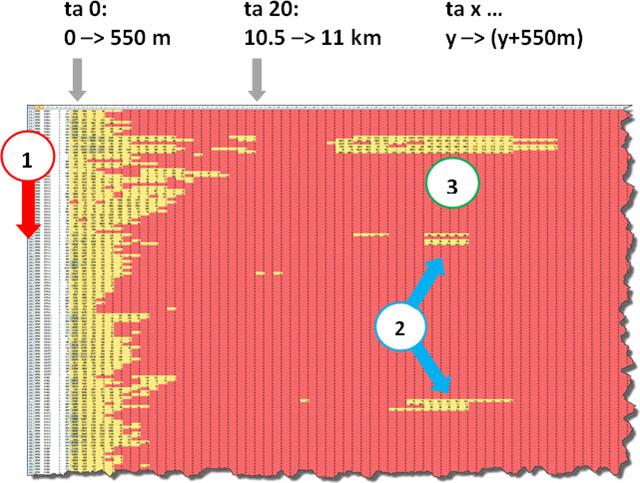
Through the information of TA for each cell, we know how far the coverage of each one is reached. So, after we change a particular tilt, simply export the new KPI data (TA), and compare the new coverage area (and also the new distributions/concentrations of traffic).
Another way, perhaps even more interesting, is plotting this data in a GIS program, for example in Google Earth. From the data counters table, and an auxiliary table with the physical information of cells (cellname, coordinates, azimuth) can have a result far more detailed, allowing precise result checking as well.
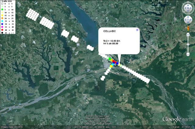
Several other interesting information can be obtained from the report (map) above.
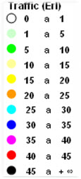
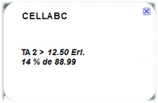
When you click some point, we have its traffic information. The color legend also assists in this task. For example, in regions around the red dots, we have a traffic between 40 and 45 Erlangs. In the same logic, light yellow points between 10 and 15 resulting Erlangs according to legend – see what happens when we click at that particular location: we have 12.5 Erlangs.
Another piece of information that adds value to the analysis, also obtained by clicking any point, is the percentage of traffic at that specific location. For example, in the yellow dot we have clicked, or 12.5 Erlangs = 14% out of a total of 88.99 Erlangs that cell has (the sum of all points).
Also as interesting information, we have the checking of coverage to far from the site, where we still have some traffic. In the analysis, the designer must take into account if the coverage is rural or not. If a rural coverage, it may be maintained (depends on company strategy). Such cases in sites located on cities, are most likely signal ‘spurious’ and probably should be removed – for example with the use of tilt!

The creation and manipulation of tables and maps processed above are subject of our next tutorial ‘Hunter GE TA’, but they aren’t complicated be manually obtained – mainly the data in Excel, which already allow you to extract enough information and help.
Conclusion
Today we’ve seen the main characteristics of tilts applied to antennas.
A good tilts choice maintains network interference levels under control, and consequently provides best overall results.
The application of tilt always results in a loss of coverage, but what one should always bear in mind is whether the reduced coverage should be there or not!
Knowing well the concept of tilt, and especially understanding the different effects of mechanical and electrical tilt, you will be able to achieve the best results in your network.
As always, we do that our last ever request: If you liked this tutorial, please share it with your friends: so you give us reason to continue publishing new articles like this! Thank you!

