Introduction
The orthogonality concept is one of the most important and crucial mechanisms that allow the existence of modern wireless systems such as WCDMA and LTE.
But not always such a concept is understood with sufficient clarity, and ends up being just ‘accepted’.
An example of this are the orthogonal codes - when it comes to CDMA and UMTS (WCDMA) we are already referring to them in the name of these access technologies itself.
In LTE we also have the fundamental role of orthogonality, only that in this case it refers to another access technology, OFDM transmission - although that is quite different from the code of CDMA and WCDMA scheme, it depends entirely on the orthogonality principle.
And that’s what we’ll study today, trying to clearly understand this principle: the orthogonality.
And for this we will demonstrate its practical application in a CDMA system. This analogy can be further extended by you in the understanding of any system that uses this principle/concept.
CDMA Example
As we will demonstrate using the CDMA technology, it is important to first do a little consideration (review) on the three most basic access technologies (FDM, TDM and CDM) with respect to bandwidth allocation and channel occupation by its users.
- In FDM (division by frequency) access: each user has a small PART OF THE SPECTRUM allocated during ALL THE TIME;
- In TDM (division by time) access: each user has ALL SPECTRUM - or nearly all - allocated at a small PART OF THE TIME;
- In CDM (division by code) access: each user will occupy ALL SPECTRUM during ALL THE TIME.
In the latter case, the multiple transmissions are identified using the theory of codes. And therein lies the great challenge of CDMA: to be able to extract the desired data at the same time we exclude all the rest - the interference, and everything that is unwanted.
These CDMA codes are called ‘orthogonal’, then let’s start with the basic meaning of this word.
What does Orthogonal means?
Seeking the origin of the word, we find that it comes from the Greek, with the first part - ‘orthos’ - meaning ‘just’, ‘righteous’, and the second part - ‘gonia’ - meaning angle.
In other words, the most common definition is: perpendicular, forming a right angle of 90 degrees between the references.
Orthogonal is a commonly used term in Mathematics (in the same way that the term Perpendicular). But there is an ‘informal’ rule: when we speak of triangles, we use the term Perpendicular, and when we refer to Geometric Vectors or Coordinates, we use the term Orthogonal.
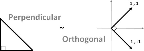
Then, according to Mathematics: if two vectors are perpendicular (the angle between them is 90 degrees), then we actually say that they are orthogonal.
Right. But how to know, through our calculations, that two vectors are orthogonal?
Let’s talk a little math, but do not worry, we will be brief.
When we talk about vectors calculations, one of the best-known operations is the Dot Product (or Scalar Product). Simply explained, it is an operation that results in a Scalar (a number) obtained by the ‘multiplying’ of two vectors. Remember that we are talking about vectors: the Dot Product multiplies each position in a corresponding position in the vector by another vector, and add all the results.
To illustrate a simple way, consider two vectors u and v with only two dimensions.
Vector u = < -3 , 2 > e Vector v = < 1, 5 >
The scalar product is equal to +7 (equivalent to -31 + 25).
This positive number, although it does not seems, already give us enough information: we will not show here, but the positive Dot Product indicates that the angle between these vectors is Acute (smaller than 90 degrees!). Likewise, if the Dot Product is negative, the angle between these vectors is Obtuse (greater than 90 degrees).
We’re almost there, and you may already be ‘connecting the dots’…
In Mathematics, another way to write the Dot Product between two vectors u and v is:
u.v = |u| |v| cos(x)
Note that now we have in the formula the information of the angle between the two vectors (the angle X). We know that orthogonal vectors has an angle of 90 degrees to each other. And we also know that the cosine of 90 degrees is equal to 0 (zero).
That is, we can conclude: if two vectors has an angle X of 90 degrees to each other - ie they are orthogonal - their Dot Product is equal to Zero!
u.v = 0
And it is from here that comes a famous definition that you may find in several literatures: ‘Two vectors are orthogonal if (and only if) the Dot Product of them is zero.’
If you failed to understand or remember the basics that you saw long time ago in school, then you now understand the algebraic operation that allows us to verify the orthogonality between vectors: the Dot Product. It is a operation between two sequences of numbers of equal length, returning a single number (the sum of the products of corresponding entries between any two sequences of numbers).
But enough math for today! We are not here to deduce or do algebraic or geometric calculations, but to understand what an ‘orthogonal signal’ is. Of course, the introduction we just saw was needed. (Note: As always we are not concerned with definitions and more complex calculations involved in this matter: you can feel free to extend in your studies).
Let’s proceed, and try to apply this orthogonality concept to our practice in the wireless networks. In this case, let’s try to understand how can we transmit multiple signals at a single frequency band, and then retrieve it.
The key here is that each of these codes do not interfere with each other. That is, these codes are orthogonal!
We say that two codes are orthogonal when the result of multiplying the two, bit-wise, over a period of time, when added is equal to Zero.
Suppose two vectors as shown below (1,1) e (1,-1). It is easy to see that they are orthogonal, no?
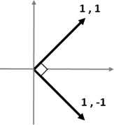
They have a right angle to each other, and the scalar product is Zero. It is easy to realize that they do not interfere with each other.
But what if we need more orthogonal codes (mutually exclusive, that do not interfere with each other)?
In this case, we need to create a set of codes (sequence of numbers) whose Dot Product is Zero. Ie, to generalize this relationship to ‘n’ dimensions where we can apply the same simple mathematical rule and verify the orthogonality.
Fortunately, a Mathematician has done all this work. Frenchman Jacques Hadamard created a simple rule to obtain a set of codes that were orthogonal - mutually exclusive.
Hadamard Matrix
To generate our mutually exclusive sequences numbers, we can follow the basic rule that the Hadamard defined in his ‘Hadamard Matrix’. In this matrix, whose entries are either +1 or -1, all rows are mutually orthogonal.
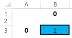
The rule of the Hadamard matrix is used for example in CDMA by the matrix that generate Walsh Codes. Let’s see how this generation would be, in a simple Excel sheet.
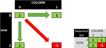
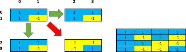
Consider the smallest and simplest existing matrix, a 1x1 matrix.
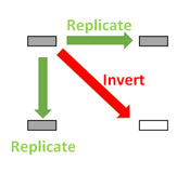
We apply this matrix rule of creation: replicate (copy matrix) to the right, replicate (copy matrix) down, and reverse (copy the inverse of the matrix multiplied by -1) diagonal.
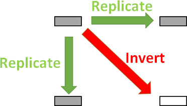
As a result, we have a 2x2 matrix.
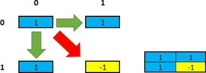
Note: see that in this case, it is still easy to notice the orthogonality in the vectors that represent these two codes.
Following the same way, now we generate a 4x4 matrix with orthogonal codes.
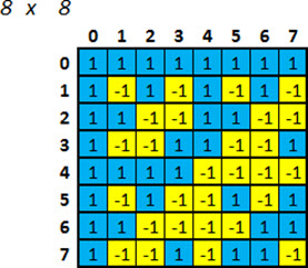
Again, we repeat the action, and now we get a 8x8 matrix.
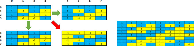
At this point, we have a matrix of 8 codes (sequence of numbers) orthogonal to each other.
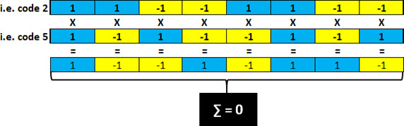
We show that the Dot Product of any line (code) for any other line (source) is always Zero. As an example, we choose the code ‘2’ and the code ‘5’. Multiplying each of the corresponding entries in each of them, we have another sequence as a result. The sum of the entries of this new resulting string is always Zero! (Do the test yourself: choose any two codes, and then multiply the corresponding entries, and sum it up: the end result is Zero! Interesting, no!?).
Okay. We understand that we can - and how we can - generate a set of orthogonal codes (sequence of numbers). But in practice, how is it all done?
Let’s continue.
Code Spreading (and Despreading)
To apply this concept to practice, we need to try to see what happens in the transmission of a spreaded signal in time: let’s see how the transmission of spreaded data works. In other words: how is it possible to many concurrent users to use exactly the same frequency, transmitting all at once, and not be a total colapse in the system?
Again, the best way to demonstrate it using examples and simple analogies.
Let’s begin by considering a signal from a particular user, with its information bits, as shown in the following figure.
Consider yet another signal, with 8 ‘carriers’ or ‘bits’.
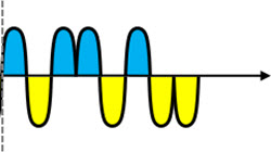
If we multiply each user information bit, for these 8 bits, we have a compound resulting signal.
This resulting signal carries the same ‘information’ that the user bits signal. But in a more ‘spreaded’ way.
When the receiver receives this resulting signal, it knows that a particular sequence represents some user information bit.
Similarly, when receiving another sequence, the receiver is able to determine that is another user information bit!
Note that for the original user bit, we now have 8 corresponding information bits arriving at the receiver. In other words: 1 bit spread in 8 ‘chips’ *!
Important: * actually, when the signal is spreaded, we do not call more than bits anymore, but chips - and this is another concept that will explain other time. When this chipstream arrives at the receiver it is properly understood by the receiver. Unfortunately the transmission in systems such as CDMA is much more complex than that. So we need to continue and try to bring this practical scenario for our study (later we can delve more).
The user’s information, which is above represented by generic bits, can be voice and/or data. Let’s represent it already as a pure digital signal, and ‘follow’ the transmission of the user bits, from its generation to its recovery at the receiver.
Transmitting (and receiving) a user’s data
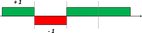
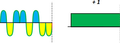
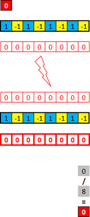
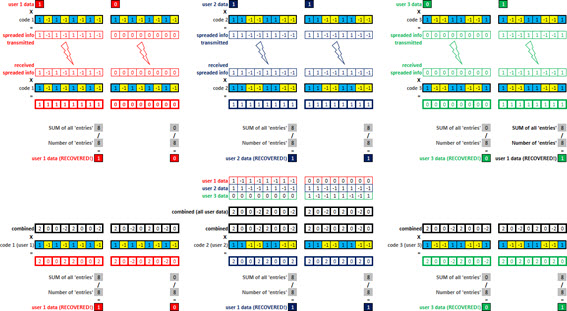
We start considering a bit of one user, first as having the value of ‘1’.
![]()
Note: in this case the red color is identifying the user 1 (and not if the bit is equal to +1 or -1). Consider as the bit value, the value that is within it - in this case equal to 1.
And now we remember what we saw earlier, about orthogonal code matrix. Let’s use an example of an array with 8 codes (ie, 8 codes are available for use, with guaranteed orthogonality among them - do not interfere with each other).
Just to make it easier to follow, we will choose the ‘Code 1’ for use with ‘User 1’ (we can choose any of the codes, doesn’t need not be ‘1’).
![]()
We then do the spreading: multiply the user one bit per each bit of code one we chose. This signal can then be transmitted, and considering initially an ideal scenario, this same sequence reaches the receiver.
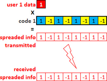
Attention that our statement now begins to get ‘interesting’: ‘How the receiver can recover the information of one user (in this case, knowing that the bit value is equal to 1?)’
The answer is simple: doing this despread of the received signal, using exactly the same code that was used to spread the signal!
Okay, still can not see how? So let’s move on.
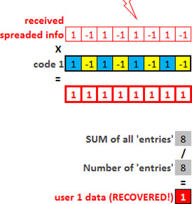
Multiply the received signal (user 1) by the same code used for spreading (code 1). As you can see, the result is a sequence of 1’s.
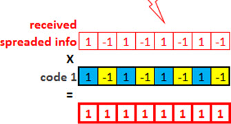
But this result is the content that has been spreaded into 8 parts. We need to add up all the information, and divide by the total of parts. In this case, the sum is equal to 8 for a total of 8 bits. Or: that information is equal to 8/8 = 1.
Okay, maybe you still have not understood well, and may think that it may have been coincidence. Okay, let’s continue.
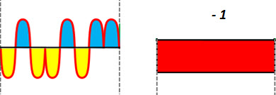
Repeat the same process, but now with the bit equal to 0. So, surprised?
Even so, you may still not be convinced.
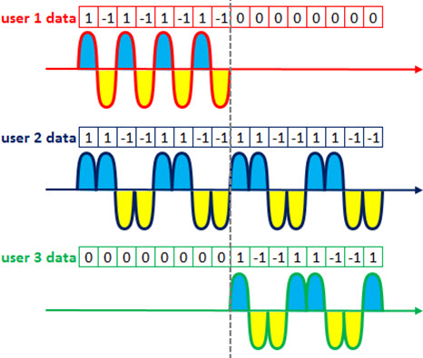
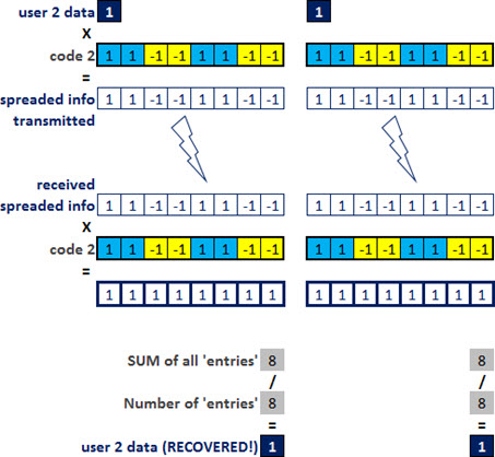
Let us now transmit new data, but now for a user 2 (we use dark blue to refer to data that user in the figures). In the theory that we have seen, for the codes/signals do not interfere with each other, they need to be orthogonal. So choose one of eight codes of our matrix of orthogonal codes that we are using as an example (let’s choose another code other than code 1, which we already use for user 1 - soon you will understand why).
Unlike the first user, who transmitted ‘10’, we now assume that the user has information on two bits equal to ‘11’. Repeating the same calculations, we have the result for user 2. Interesting, no?
Even with the demonstrations above, if you’re still not convinced that the division can be done by code, see an example for a third user (green), sending ‘01’.
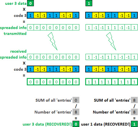
We could stay here with endless demonstrations, but we believe that you already understood the idea, didn’t you?
Right. So enjoy a little breathing because the best is yet to come.
As we are trying to learn today, one of the main functions of these types of codes that we used above is to preserve orthogonality among different communication channels.
From the set of orthogonal codes obtained from the Hadamard matrix, we can make the spread in communication systems in which the receiver is perfectly synchronized with the transmitter, generating codes according to the characteristic of each system.
So far so good. In the example above, we have spreaded, transmitted and recovered the user data. But individually! In practice, the data of each user are not transmitted separately, but all at the same time!
The highlight, the great advantage of the transmission using codes is precisely the ability to transmit multiple users the same time (using orthogonal codes) and extract the data for each user separately!
Again, through examples is easier to visualize how this works. So let’s continue?
Transmitting (and receiving) data of multiple users
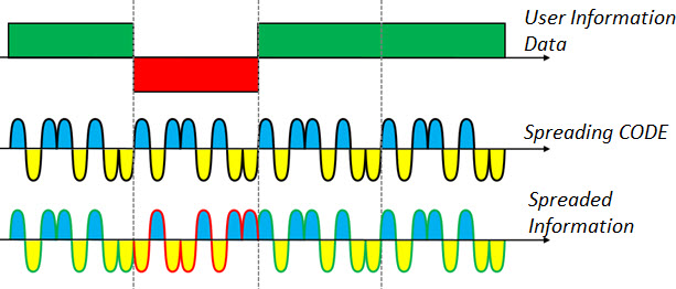
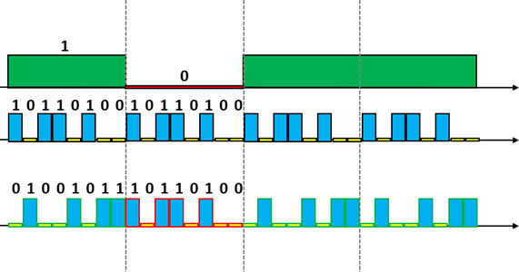
Suppose then all previously spreaded signals arriving at the receiver.
We can represent these signals as waveforms, so it is easier to view them.
And the composite signal can be represented in the same way (the incoming signal is always the sum of all signals of each user).
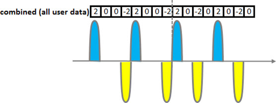
Take a little break here: the composite signal (shown above) is the sum of all the spreaded signals from all users, and apparently doesn’t give us any interesting information, right?
Wrong. Actually, the above statement is only apparent: in fact, we have a lot of information ‘carried’ in one signal.
Let’s continue. Looking only at the composite signal, we have no idea what is ‘clustered’. This is normal, and it really is what it ‘seems’.
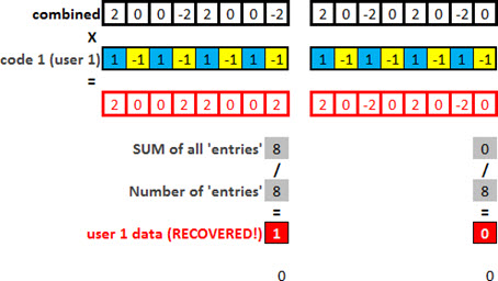
But now let’s go back to the theory that we learn of orthogonal codes: when we multiply a code by another code, all that is not orthogonal is interference, and should be excluded.
Ie if we multiply an orthogonal code for this set of codes, we have to split or ‘recover’ that information back.
So if we multiply the orthogonal code used to spread the signal of user 1, we obtain the original signal of user 1!
Magic? No: simply Engineering, Mathematics and Physics!
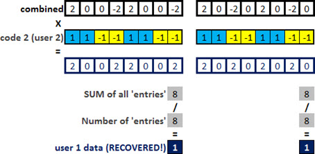
We can do the same with the user 2: use the same unique spreading code, and obtain the original signal!
Similarly, the same with the third user.
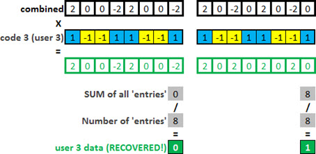
And it doesn’t matter how many users are there: if they were spreaded using orthogonal codes they can be despreaded the other way, with the same unique code for each one!
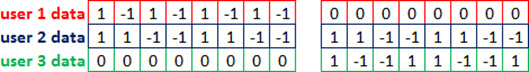
The following figure illustrates the general summary of everything we saw today (even if the font is too small,it serves to show the generic scenario).
Congrats! You just prove that dividing signals using codes is actually possible, and that CDMA works!
Orthogonality in LTE and GSM
We did understand and apply the concept of orthogonality in orthogonal codes used in CDMA and WCDMA systems.
But in other systems, how does it work?
In fact, and as mentioned before, all systems rely on some type of orthogonality to work, ie some way of transmitting information so that it can be retrieved (as shown today).
However, due to the characteristics of each system, this concept applies differently.
As our tutorial is already quite extensive for today, let’s not over extend ourselves, and we will cover this topic in the future, in tutorials that require this prior understanding.
Ideal World x Real World
It is also clear that not everything is perfect: in our example, we consider an ideal world without interference or any other problem that could affect our communication. Unfortunately, they exist, and quite a lot!
For example the codes are orthogonal only - not interfere with each other - if they are perfectly synchronized. In our example, we do not consider the phase difference between them - in other words, we consider the light speed to be infinite.
There is also the effect of the multipath components, which makes this recovery of the signal much more complex that shown in the simplifications we’ve seen.
But they all have its solutions. Most refers to common problems, problems grouped as ‘Multi-User Detection’, which in turn have a number of techniques to minimize each of these effects. The Rake Receiver already explained in another tutorial is one of them.
We still factors like Power Control, which would have different ‘weights’ for each user. And a number of other factors and limitations of all types to further complicate this communication.
Naturally, all these complications have solutions, and that is fantastic task at a Telecom Professional faces in its day-to-day.
But for today, we believe that what we’ve is enough, at least for the clear understanding of the basic principle of orthogonality - which was our initial goal, remember?
Physical x Logical Mapping
To conclude, in the demonstrations we’ve used examples codes with 8 bits (remembering that in fact, when the signal is spreaded we do not call it bits, but chips instead; this is the subject of another tutorial, and let’s not to lose our focus today), when in reality they are much bigger, as 64 Walsh Codes in CDMA.
We used addition and multiplication operation, because we considered the physical signals in their physical layer: when signals are mapped to the physical layer, we assign them bipolar values - in our case, +1 and -1.
But in logical operations we have 0’s and 1’s. And in this case, we use the binary XOR operation. (We are already well advanced by now, and let’s not extend ourselves to that subject - which already would require another tutorial just to explain in a simplified way).
Simply understand that the codes used by systems such as CDMA and WCDMA are also Type 0’s and 1’s. In the XOR operation: if the bits are equal, the result is 0. If the bits are different, the result is 1.
When we applied XOR to any different Walsh code (or any other set of orthogonal codes), the result is always half 0, and half 1 (in the Hadamard matrix, so that the sum is 0, half is equal to +1, and half is equal -1).
And when we apply XOR to equal codes, the result is only 0’s!
Although it seems simple, this operation allows the system to work perfectly.
The following is an example of a Walsh code matrix with 64 orthogonal codes used in CDMA.
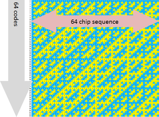
As an example for UMTS, we can mention OVSF (Orthogonal Variable Spreading Factor) codes, virtually identical to the Walsh codes (CDMA IS-95) - only that the generation is different.
We’ll also talk about these specific codes in other tutorials, explaining how they are used for different channeling.
Now: enough for today, do you agree?
As you can see, we have plenty of themes or topics to explore and explain a simple way to make you extract the maximum possible in your learning program, and also when apply it to your work. We’ve seen many concepts for today!
If you managed to understand well at least the concept of orthogonality, and how it makes it possible the code division to happen, it is definitely enough. In later tutorials we will continue addressing other concepts, and trying to show them in the most simplified manner.
IMPORTANT: we did not talked too much about chips and symbols today, but it is directly related to the subject. Anyway, they were not essentially the subject today.
Again, as always: all of these concepts that were not covered today will be detailed in other tutorials.
Conclusion
Today we knew one of the most basic concepts, but also one of the most important, which makes possible the existence of modern wireless networks: the orthogonality concept.
As an example, we saw how the concept applies in practice to CDMA and WCDMA systems, more specifically in the form of orthogonal codes applied to the physical system, allowing the access division by codes to happen, and thus achieving multiplexing of different chipstreams of users in the same carrier without inserting interference therebetween.
The concept is much broader than what we try to show here today, and extends to many other areas and technologies. Anyway, we hope it can be helpful for the further development in the subject.
telecomHall Community
![]() Telecom Made Easy!
Telecom Made Easy! ![]()
(Share to your friends ![]() )
)