OTN Learning Series Part 6: OTN Mapping Vs Grooming

[OpticRoute]

𝗧𝗵𝗲 𝗗𝗶𝗳𝗳𝗲𝗿𝗲𝗻𝗰𝗲 𝗠𝗼𝘀𝘁 𝗘𝗻𝗴𝗶𝗻𝗲𝗲𝗿𝘀 𝗠𝗶𝘀𝘀

Many engineers use the words 𝗺𝗮𝗽𝗽𝗶𝗻𝗴 and 𝗴𝗿𝗼𝗼𝗺𝗶𝗻𝗴 interchangeably.

They are not the same.

If you confuse them, you misunderstand how OTN actually works.

---

𝗪𝗵𝗮𝘁 𝗢𝗧𝗡 𝗠𝗮𝗽𝗽𝗶𝗻𝗴 𝗥𝗲𝗮𝗹𝗹𝘆 𝗜𝘀

𝗠𝗮𝗽𝗽𝗶𝗻𝗴 is the act of placing a client signal into an OTN container.

It happens at the 𝗢𝗣𝗨 layer.

You take:

10GbE 100GbE SONET OC 192

And you adapt it into structured payload.

Mapping answers one question:

Where does this signal live inside OTN?

It does not combine services. It does not switch containers. It does not optimize capacity.

It simply adapts and inserts.

---

Figure 6.1

Client signal entering OPU and becoming structured OTN payload.

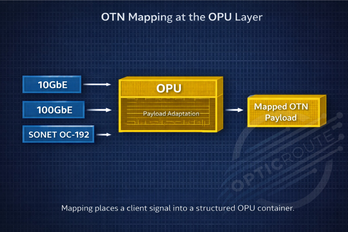
Figure 6.1

---

𝗪𝗵𝗮𝘁 𝗢𝗧𝗡 𝗚𝗿𝗼𝗼𝗺𝗶𝗻𝗴 𝗥𝗲𝗮𝗹𝗹𝘆 𝗜𝘀

𝗚𝗿𝗼𝗼𝗺𝗶𝗻𝗴 happens at the 𝗢𝗗𝗨 layer.

It is switching and aggregation of containers.

Example:

10 x ODU0 services Mapped into 1 x ODU2

Or

Multiple ODU2 Aggregated into ODU4

Grooming answers a different question:

How do we efficiently transport multiple services across the backbone?

It involves:

𝗢𝗗𝗨 𝘀𝘄𝗶𝘁𝗰𝗵𝗶𝗻𝗴 𝗛𝗶𝗲𝗿𝗮𝗿𝗰𝗵𝗶𝗰𝗮𝗹 𝗺𝘂𝗹𝘁𝗶𝗽𝗹𝗲𝘅𝗶𝗻𝗴 𝗦𝗲𝗿𝘃𝗶𝗰𝗲 𝗮𝗴𝗴𝗿𝗲𝗴𝗮𝘁𝗶𝗼𝗻

This is where transport engineering becomes architectural.

---

Figure 6.2

Multiple ODU containers entering an OTN cross connect and merging into higher rate container.

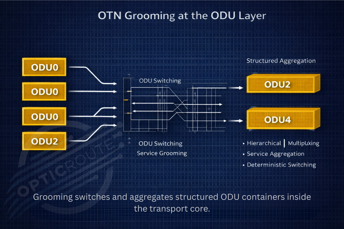
Figure 6.2

---

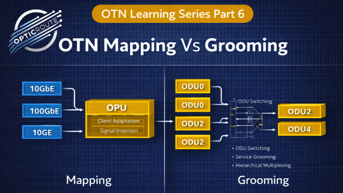
𝗠𝗮𝗽𝗽𝗶𝗻𝗴 𝗩𝘀 𝗚𝗿𝗼𝗼𝗺𝗶𝗻𝗴 𝗦𝗶𝗺𝗽𝗹𝗶𝗳𝗶𝗲𝗱

Here is the clean distinction:

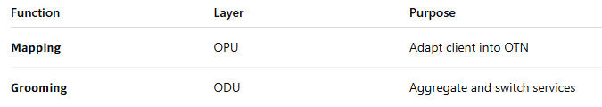
Mapping is vertical. Client into container.

Grooming is horizontal. Container to container.

One prepares the signal. The other optimizes the network.

---

Figure 6.3

Side by side comparison showing mapping flow versus grooming flow.

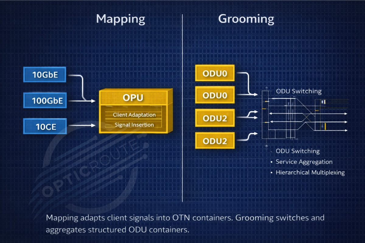
Figure 6.3

---

𝗪𝗵𝘆 𝗧𝗵𝗶𝘀 𝗗𝗶𝘀𝘁𝗶𝗻𝗰𝘁𝗶𝗼𝗻 𝗠𝗮𝘁𝘁𝗲𝗿𝘀

If you mislabel mapping as grooming:

You oversimplify network design. You misunderstand OTN cross connects. You confuse service adaptation with service optimization.

In large backbone deployments, that confusion leads to:

Poor capacity planning Inefficient hierarchy usage Operational complexity

Transport engineering demands precision.

𝗠𝗮𝗽𝗽𝗶𝗻𝗴 is about structure. 𝗚𝗿𝗼𝗼𝗺𝗶𝗻𝗴 is about scale.

Both are essential. But they solve different problems.

---

Figure 6.4

End to end flow showing client mapping at ingress and grooming in core network.

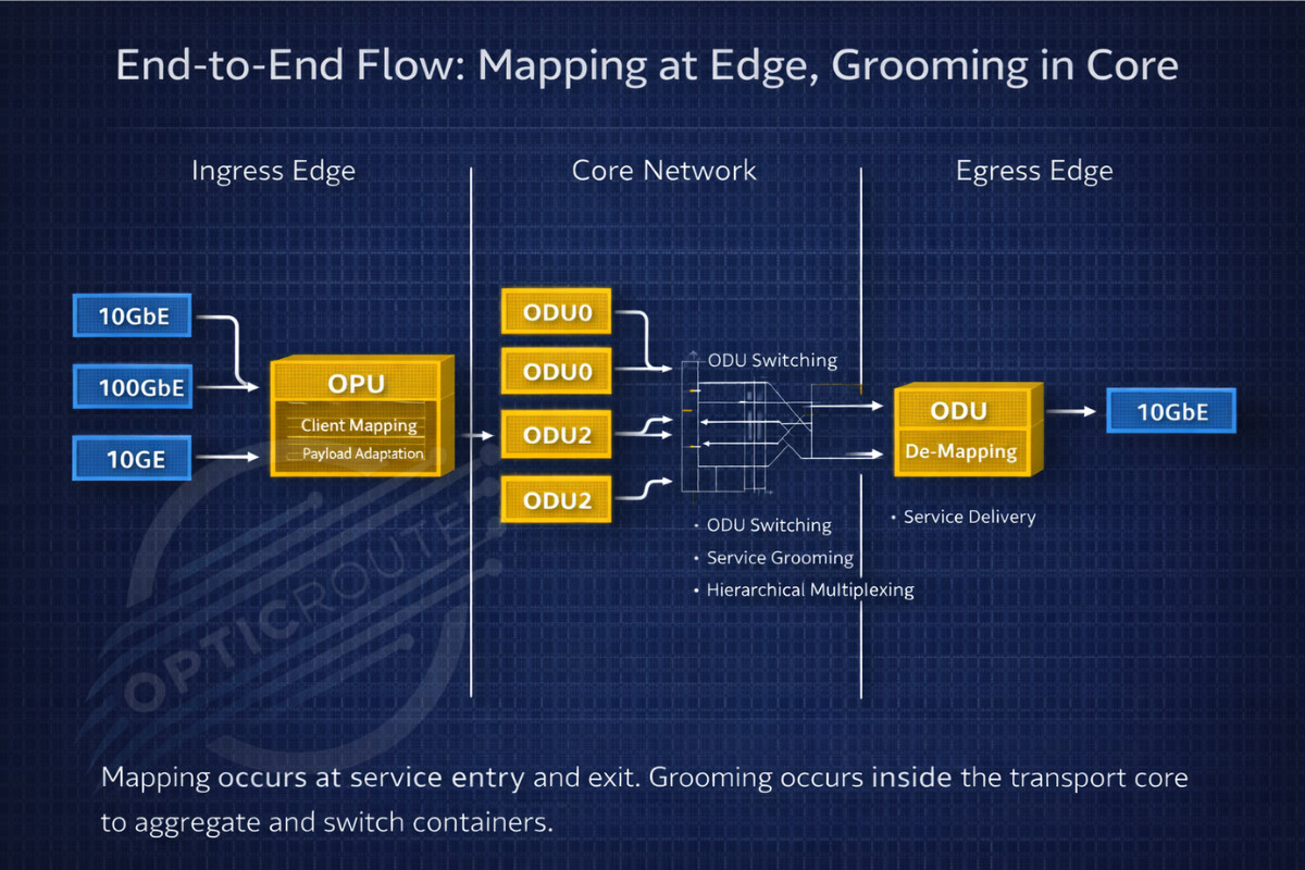
Figure 6.4