OTN Learning Series Part 5: OTN Rates and Containers

[OpticRoute]

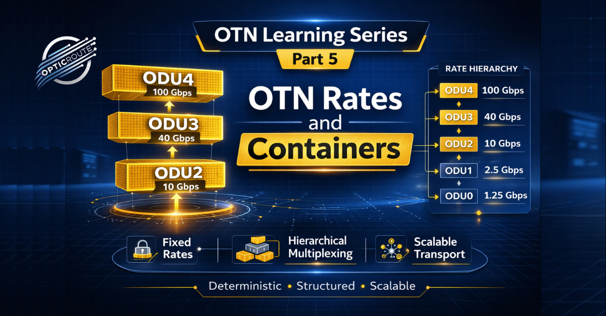
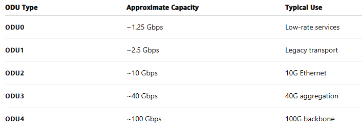
Most engineers first encounter OTN rates as a table of numbers.

ODU0

ODU1

ODU2

ODU3

ODU4

It feels like memorization.

It is not.

𝗢𝗧𝗡 𝗿𝗮𝘁𝗲𝘀 𝗮𝗿𝗲 𝗮𝗯𝗼𝘂𝘁 𝘀𝘁𝗿𝘂𝗰𝘁𝘂𝗿𝗲.

Once you understand the structure, the numbers make sense.

---

𝗧𝗵𝗲 𝗕𝗮𝘀𝗶𝗰 𝗜𝗱𝗲𝗮

OTN defines fixed-rate containers called 𝗢𝗗𝗨𝗸.

Each ODUk represents a specific payload capacity.

Think of them as standardized transport boxes.

Here are the core ones you will see in modern networks:

These are fixed containers.

They do not float. They do not burst. They are deterministic.

---

𝗢𝗗𝗨𝗸 𝗖𝗼𝗻𝘁𝗮𝗶𝗻𝗲𝗿 𝗛𝗶𝗲𝗿𝗮𝗿𝗰𝗵𝘆

ODUk containers are scalable building blocks.

Higher containers can carry multiple lower containers through multiplexing.

Example:

• Multiple 𝗢𝗗𝗨𝟬 can fit into 𝗢𝗗𝗨𝟮

• Multiple 𝗢𝗗𝗨𝟮 can be mapped into 𝗢𝗗𝗨𝟰

This is structured aggregation, not statistical sharing.

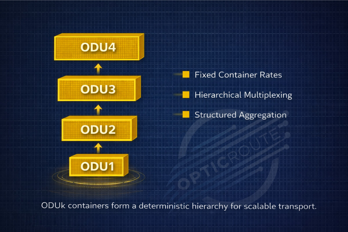
Figure 5.1: ODUk Container Hierarchy

---

𝗙𝗹𝗲𝘅𝗶𝗯𝗹𝗲 𝗚𝗿𝗶𝗱 𝗮𝗻𝗱 𝗢𝗗𝗨𝗳𝗹𝗲𝘅

Modern OTN goes further with 𝗢𝗗𝗨𝗳𝗹𝗲𝘅.

ODUflex allows bandwidth to be allocated in smaller time-slot increments.

Instead of being locked to rigid 10G or 100G blocks, you can create:

• 25G services

• 75G services

• Custom bandwidth profiles

But here is the important distinction:

Even with ODUflex, bandwidth is still explicitly assigned.

It is not shared dynamically like Ethernet.

---

𝗢𝗗𝗨𝗳𝗹𝗲𝘅 𝗕𝗮𝗻𝗱𝘄𝗶𝗱𝘁𝗵 𝗔𝗹𝗹𝗼𝗰𝗮𝘁𝗶𝗼𝗻

ODUflex slices time slots inside a higher-rate container.

Each slice is controlled.

Each slice is monitored.

Each slice is deterministic.

Figure 5.2: ODUFlex Bandwidth Allocation

---

𝗥𝗮𝘁𝗲𝘀 𝗮𝗿𝗲 𝗡𝗼𝘁 𝗔𝗯𝗼𝘂𝘁 𝗦𝗽𝗲𝗲𝗱

This is where many engineers misunderstand OTN.

OTN rates are not primarily about speed.

They are about:

• 𝗦𝘁𝗿𝘂𝗰𝘁𝘂𝗿𝗲

• 𝗦𝗰𝗮𝗹𝗮𝗯𝗶𝗹𝗶𝘁𝘆

• 𝗠𝘂𝗹𝘁𝗶𝗽𝗹𝗲𝘅𝗶𝗻𝗴 𝗯𝗼𝘂𝗻𝗱𝗮𝗿𝗶𝗲𝘀

• 𝗦𝗲𝗿𝘃𝗶𝗰𝗲 𝗶𝗱𝗲𝗻𝘁𝗶𝘁𝘆

When you design a backbone, you are not asking:

How fast is this link?

You are asking:

How are services structured inside this link?

That question leads you to the correct ODU level.

---

𝗙𝗶𝗻𝗮𝗹 𝗠𝗲𝗻𝘁𝗮𝗹 𝗠𝗼𝗱𝗲𝗹

𝗢𝗗𝗨𝗸 𝗮𝗿𝗲 𝗳𝗶𝘅𝗲𝗱 𝗰𝗼𝗻𝘁𝗮𝗶𝗻𝗲𝗿𝘀. 𝗢𝗗𝗨𝗳𝗹𝗲𝘅 𝗶𝘀 𝗰𝗼𝗻𝘁𝗿𝗼𝗹𝗹𝗲𝗱 𝗳𝗹𝗲𝘅𝗶𝗯𝗶𝗹𝗶𝘁𝘆.

Both operate under deterministic transport rules.

That is the difference between:

𝗧𝗿𝗮𝗻𝘀𝗽𝗼𝗿𝘁 𝗲𝗻𝗴𝗶𝗻𝗲𝗲𝗿𝗶𝗻𝗴

and

𝗧𝗿𝗮𝗳𝗳𝗶𝗰 𝗲𝗻𝗴𝗶𝗻𝗲𝗲𝗿𝗶𝗻𝗴

---

In 𝗣𝗮𝗿𝘁 𝟲, we will go deeper into 𝗢𝗧𝗡 𝗺𝘂𝗹𝘁𝗶𝗽𝗹𝗲𝘅𝗶𝗻𝗴 and time-slot architecture, where the real design decisions happen.