First, take a look at this diagram
Industry professionals will immediately recognize this—it’s the MR triangulation positioning!
Before diving into the main content, let’s clear up some basics: What exactly is triangulation positioning?
It calculates the distance between the terminal and base stations using MR data from multiple base stations, then draws circles using the base station coordinates to determine intersection points, thereby obtaining the terminal’s coordinates. This is a simplified description of the MR positioning process; of course, the actual calculation is far more complex.
Technical Principles of MR Positioning
MR positioning is based on mobile network measurement reports. It calculates the distance between terminal devices and base stations through parameters such as RSRP (Reference Signal Received Power) and TA (Timing Advance), then combines base station geographic coordinates using geometric algorithms (such as interpolation or circle intersection) to determine the UE’s (User Equipment) position at that time.
Core steps include: data loading and field mapping (compatible with different data formats), distance calculation via path loss models, neighbor cell filtering, distance computation, coordinate positioning, AOA (Angle of Arrival) correction, result aggregation, and Geohash encoding:
-
Inputs
- MR data including serving cell/neighbor cell engineering parameters (latitude/longitude, antenna height, etc.), measurements (RSRP, TA, CRSP, frequency/ARFCN, AOA, etc.)
-
Distance
- First, convert “measurement strength → distance”: Use path loss models to estimate slant range from RSRP, CRSP, frequency, etc., then combine with height to obtain horizontal distance; some scenarios also use TA and height-related geometric relationships (code logic implemented in series across various algorithm sub-modules)
-
Position
- On the horizontal plane, treat each cell as a circle center with estimated distance as radius:
- Interpolation Method: Perform linear interpolation along the line between serving cell and neighbor cells, using the ratio of horizontal distances on both sides
- Circle Intersection Method: Calculate pairwise circle intersections from multiple cells, then apply configured fusion strategies (such as minimum residual, weighted centroid, least squares, etc.) to obtain coordinates; fallback to interpolation when neighbor cells are insufficient or geometric degradation occurs
- On the horizontal plane, treat each cell as a circle center with estimated distance as radius:
-
AOA Correction
- Apply direction/projection-based corrections to coordinates using AOA (optional operation, independently controlled from main algorithm)
The complexity of algorithm implementation affects both positioning accuracy and system performance.
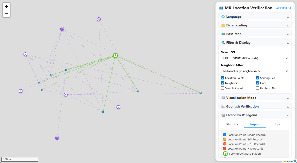
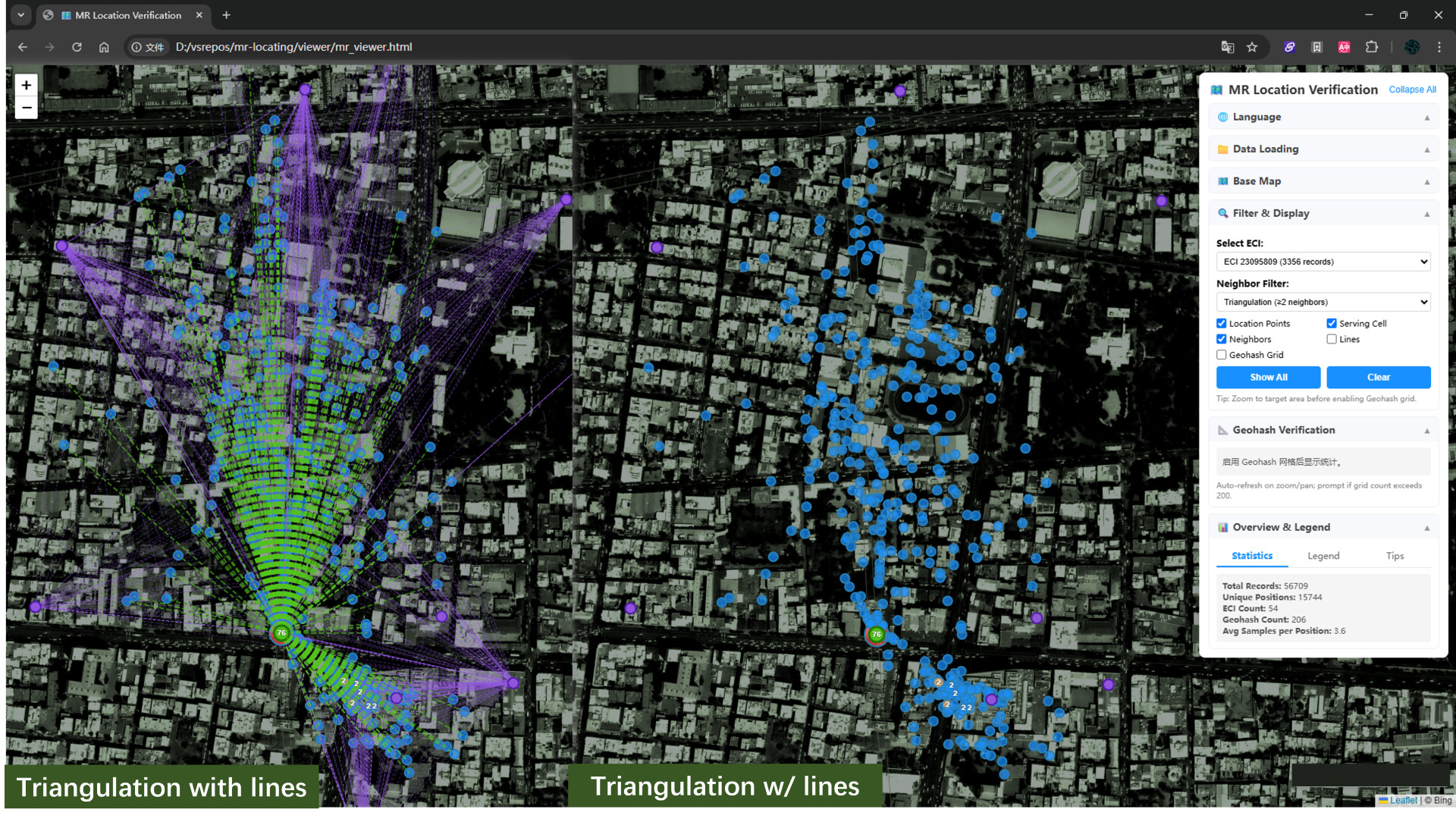
After completing the positioning process, selecting one base station’s MR dataset and visualizing the positioning results on a map produces this effect—green represents the serving cell base station, purple represents neighbor cell base stations, with lines indicating measurement relationships.

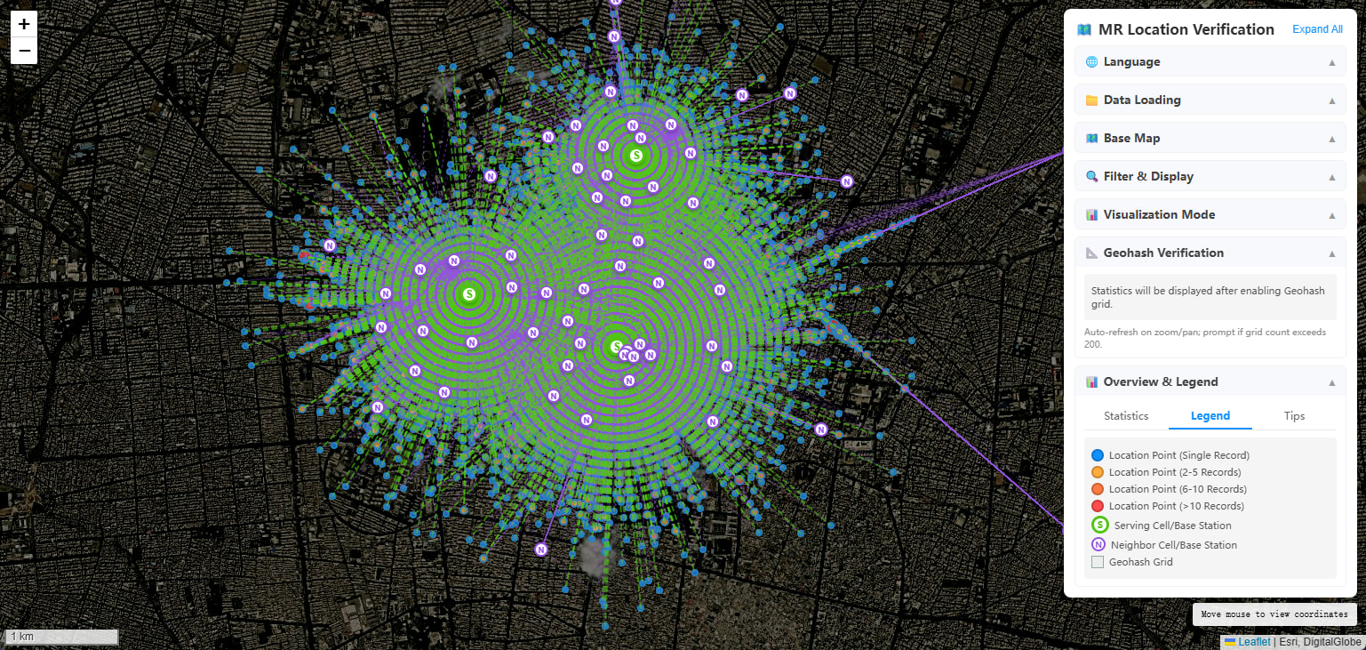
This is just a few hundred data points from one base station. When rendering over 100,000 points from a single data file on the map, the browser would instantly become unresponsive, requiring more than ten minutes to recover!
This was unacceptable, so GPU acceleration was implemented. Now over 100,000 points open instantly; only when enabling connection lines is there a slight wait. Previously, zooming the map required several minutes of waiting—now operations are smooth with silky rendering.
Positioning Algorithms and Application Scenarios
The entire positioning process involves combinations of multiple algorithms, with the path loss model being the most critical—other algorithms serve auxiliary functions.
-
Interpolation Algorithm
- Calculates UE position based on linear interpolation between serving cell and individual neighbor cells. Application scenarios: Limited neighbor cells (1-2), simple scenarios; fast computation but accuracy depends on the distance ratio between the two cells.
-
Circle Intersection Algorithm
- Uses intersections of distance circles from multiple neighbor cells for triangulation positioning. Application scenarios: Multiple neighbor cells (3+) available, high-precision requirement scenarios; improves positioning accuracy through measurement event grouping and fusing multiple intersection points.
-
Fusion Methods
- Supports Weighted Centroid and Residual Minimization for final fusion of multiple candidate positions.
-
Path Loss Models (determines “distance” quality)
- FSPL, Cost231 (urban/suburban/rural), Macro (urban/rural), Walfisch-Ikegami (can be triggered for canyon scenarios)
- FSPL: Simple, consistent with legacy versions
- Cost231/Macro: More aligned with cellular macro-station propagation classification
- WI: Complex propagation in urban streets/canyons, requires parameter tuning
-
RSRP Distance Correction
- none / ratio / weighted, etc.; can constrain ratio upper/lower bounds; optional correction for serving side when NR lacks TA. Used when path loss deviates significantly from actual measurements or when NR lacks TA.
-
AOA Correction
- Switch + weight + alignment threshold.
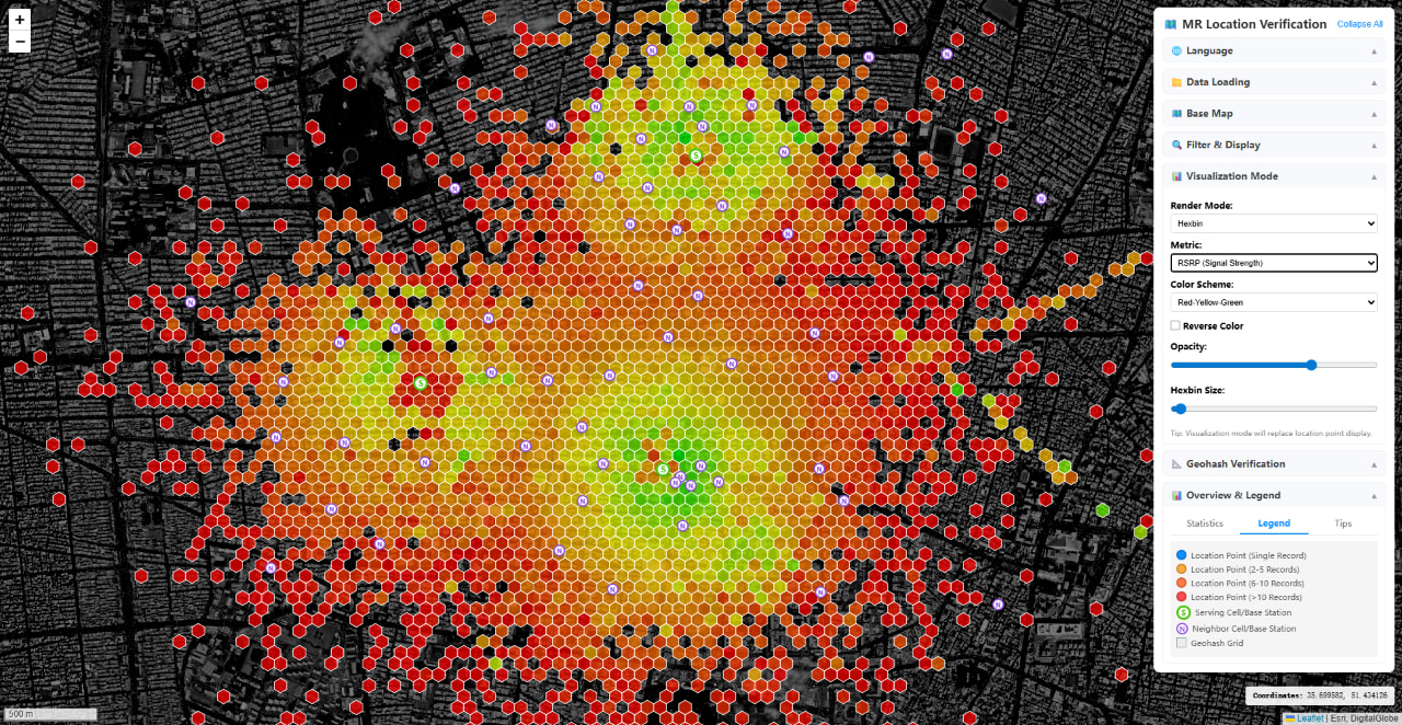
After obtaining positioning results, network metrics can be rendered on GIS maps to support various application analyses.
Using positioned measurement metrics to generate a rendered map for coverage quality analysis—this is an RSRP Hexbin grid rendering, clearly showing the base station’s “under-the-tower blackout” effect!
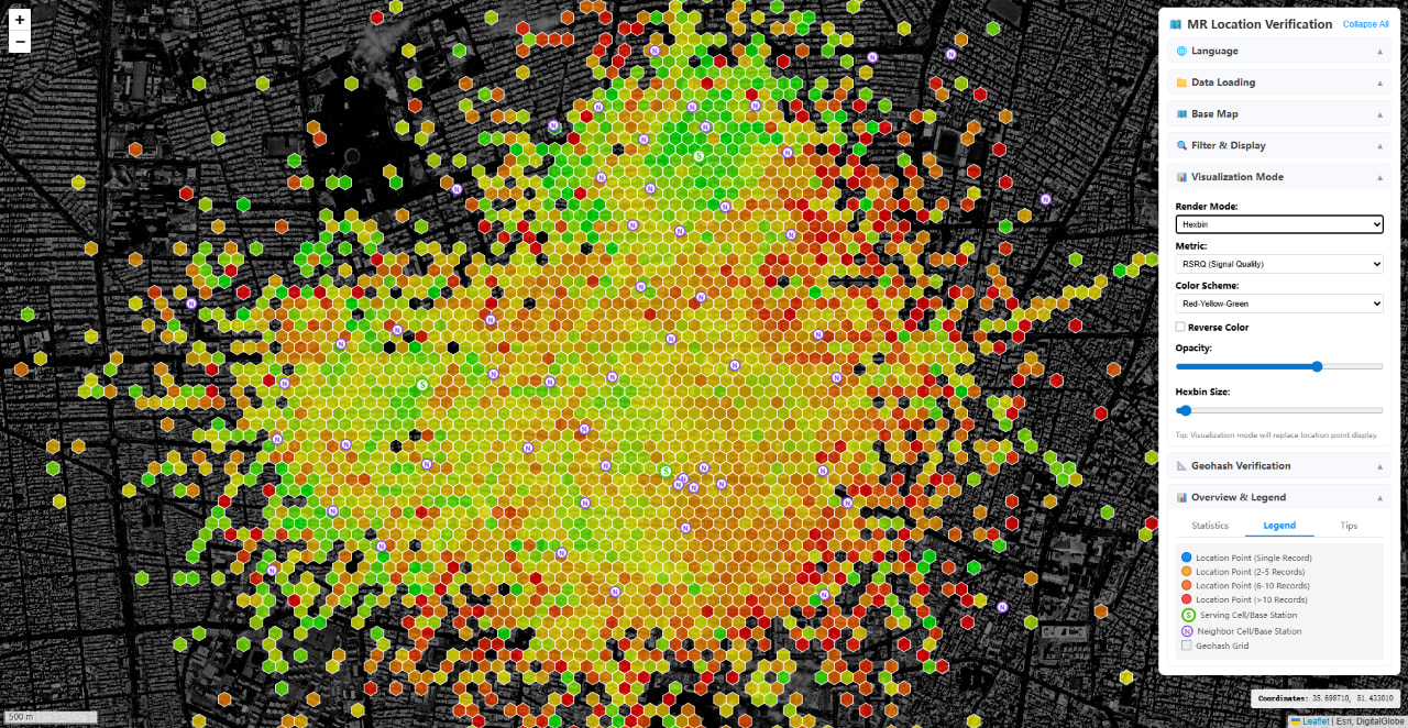
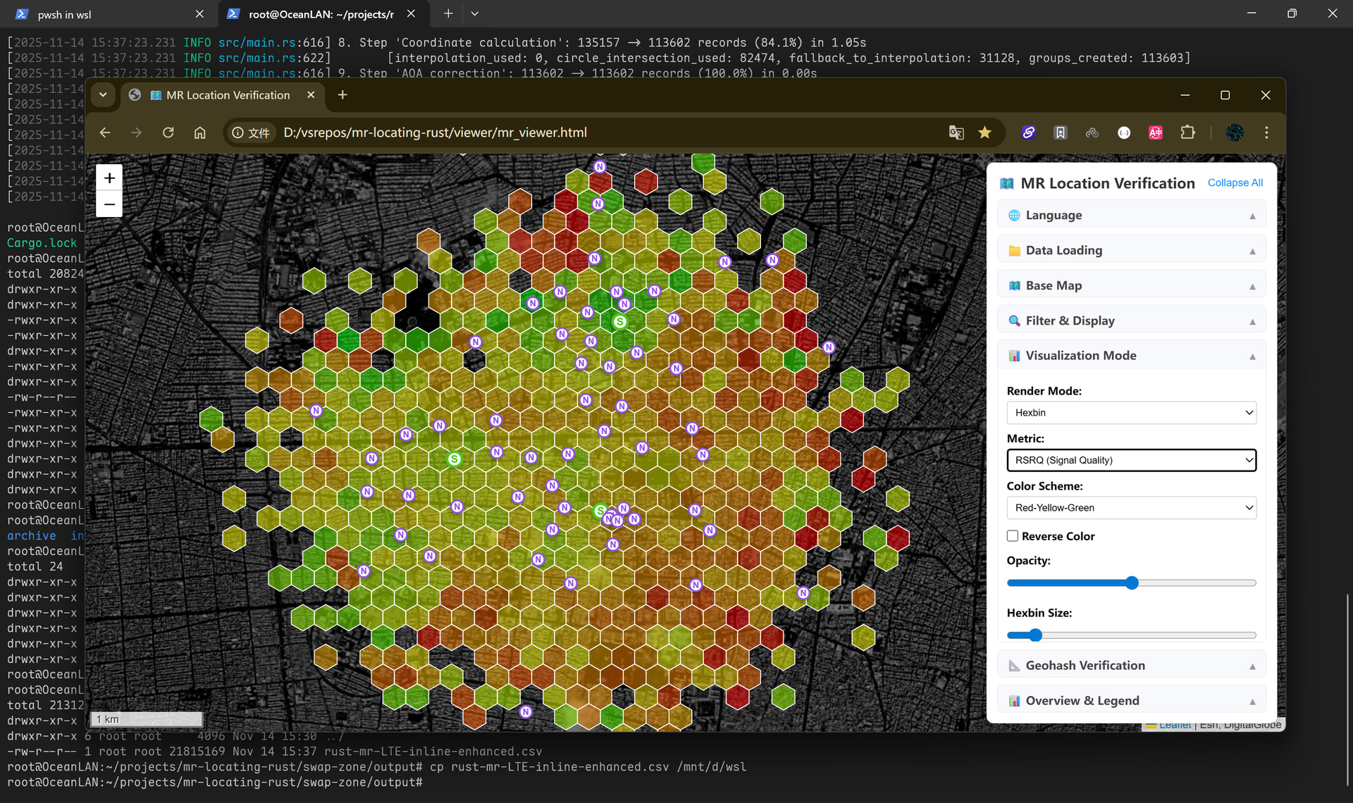
Now let’s try RSRQ—also Hexbin grid rendering. From the rendered map, we can see that coverage quality in the northwest region is noticeably better than in the southeast.
Parameter Optimization for Positioning Accuracy
-
Path Loss Models
- Macro, Cost231, FSPL, Walfisch-Ikegami (WI)—affects RSRP-to-distance conversion accuracy. Corresponding configuration parameters:
path_loss_model,path_loss_wi_trigger, full Walfisch–Ikegami set (LOS, city size, Hb/Hm, street width, building height, orientation angle, etc.)
- Macro, Cost231, FSPL, Walfisch-Ikegami (WI)—affects RSRP-to-distance conversion accuracy. Corresponding configuration parameters:
-
Power and Measurements
default_crsp_dbm,rsrp_correction_methodandratio_*,ratio_apply_to_serving_without_ta,tx_pwr_estimation_enabled(behavior when CRSP/TA is missing)
-
AOA Correction Parameters
- Weight (default 0.3), alignment threshold (default 45 degrees)—used for angle-assisted positioning
-
Neighbor Cell Filtering Parameters
- Maximum neighbor cells (default 5), minimum distance threshold (default 1 meter, for filtering co-site neighbor cells)
-
Geometry and Neighbors
max_neighbors,min_distance_meters, neighbor cell filtering and sorting (affects the point set participating in circle intersection/interpolation)
-
Circle Intersection Side
use_circle_intersection,fusion_method,fusion_weighting, and least squares-related step size/iterations
-
AOA Correction
enable_aoa_correction,aoa_weight,aoa_alignment_threshold_deg
-
Data Quality
skip_invalid_arfcn_records, whether frequency conversion is correct, etc.
-
Output Granularity
time_window_seconds(aggregation changes event semantics),geohash_precision(display/grid precision—not directly equal to physical precision but affects downstream usage)
-
Other Parameters
- Default CRSP (15 dBm), antenna height (15 meters), Geohash precision (7 digits), time window aggregation, etc.
Path loss models must be selected based on coverage type, so the objects of parameter optimization are those non-model parameters. Additionally, there’s a more practical issue: base station engineering parameters have an even greater impact on positioning accuracy.
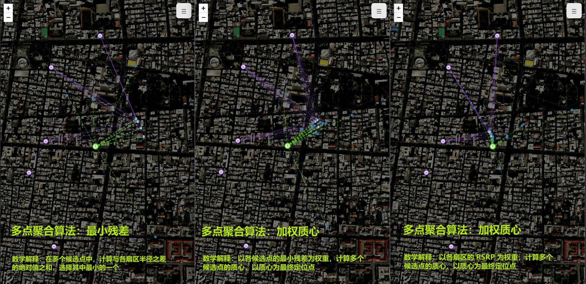
For multiple positioning results requiring aggregation algorithms, the comparison chart below shows that output results from different aggregation algorithms exhibit significant differences. Therefore, field drive test verification is needed to select the more suitable aggregation algorithm.
In MR datasets, the difference between having many neighbor cells versus few is also quite evident. At least two neighbor cells are required to qualify as triangulation positioning; otherwise, the positioning result is merely interpolation along the line between two base stations.

Furthermore, there’s AOA correction—selecting results with smaller errors based on angle of arrival.
After numerous rounds of optimization, positioning accuracy has been significantly improved. The diagram below shows which base station each positioning result’s measurement report originates from.
![]()
Data Visualization
When using data visualization tools to validate positioning results, it’s necessary to select samples separately for different base station types and neighbor cell count combinations to inspect and verify calculation results.
In this diagram, we can see that one serving cell may have dozens of neighbor cells, with hundreds of positioning results scattered across the regions between these dozens of neighbor cells. In very early versions, due to parameter issues, these positioning points would exhibit concentrated distributions at specific locations (such as the serving base station) or specific routes (serving-neighbor base station connection lines). After algorithm refinement, these issues have been resolved, and abnormal distributions no longer occur.
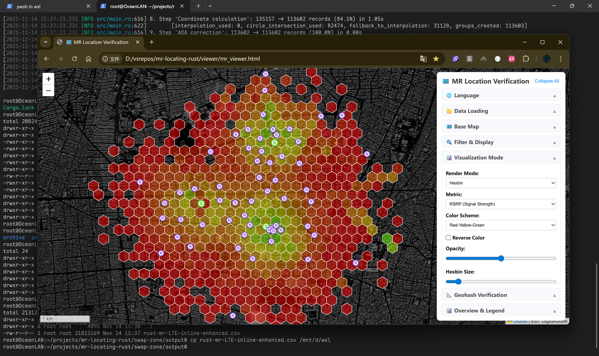
When aggregating over 100,000 positioning results by sector for GIS rendering, Hexbin grid rendering was adopted rather than the square GRID rendering commonly used by many peers—the latter looks like mosaic and always feels somewhat off. The honeycomb grid style better aligns with the essence of cellular systems.
First tried RSRP, now let’s see RSRQ results.
System Performance Indicators
-
Carrier-Grade High Efficiency
- MTPS-level positioning processing; single server achieves real-time processing of over 1 million MR records
-
Multi-Network Compatibility
- Supports various cellular network standards; compatible with and adaptable to different MR data format standards
-
Production-Grade Reliability
- Memory safety checks, error retry, state persistence, graceful shutdown; supports service mode with continuous monitoring
-
High-Precision Positioning Algorithms
- Supports circle intersection triangulation, multiple path loss models, RSRP correction, AOA correction; parameters tunable by city/scenario; positioning accuracy configurable and optimizable
Welcome friends with project cooperation opportunities to contact us through the official account backend!