Introduction
Moving forward in the creation of our entire System for our Network Monitoring and Analysis, today we’ll see the next step: defining the KPI Base Tables.
These tables are extremely important, as it will be from it we’ll create several applications, using algorithms and intelligence. From these tables, we easily create charts and dashboards, reports, and all that is necessary for a quick and efficient analysis, always following our simplified methodology.
Note: Again, remember that some concepts that we use here have been exposed in detail in other tutorials. Therefore, for a better follow-up, if you still didn’t read those tutorials, do so before proceeding.
Why store the KPI’s in Tables?
We’ve already answered this question before, but basically for two reasons: the data are already in the format ready to be analyzed, and we also have a processing gain, since the table already has the key Indicators that we use already calculated.
Moreover, we can store in tables with more than one granularity. Explaining the principle we have one table with indicators for each cell. But we need to report in other granularities, such as the indicators for all cells in the same time (system). Of course this course can be done via a query, properly grouping the data, and doing the calculations - additions, multiplications, divisions, etc…
But as we often need to use these summaries grouped, it’s a good idea to store this data in specific tables. Then, when needed, their info are already available.
Granularities of Tables
At first, we have several granularities, or clusters. Let’s now define three main granularities.
- CELL : each record (line) has information of a sector or cell.
- BSCRNC : summary of indicators grouped by BSC / RNC. This table no longer has the CELL field. For each BSC / RNC, we have the overall indicators.
- NET : Summary Indicators for the System (entire Network).
Note: There is much smaller granularities, eg TRX (GSM) and carrier (UMTS). We will address this issue later.
In addition, we have another common field in all tables that informs the technology (‘Technology’). But for now, we don’t need to worry about it.
Other granularities can be created, always following the same structure and procedures, as well as by BTS / NodeB. These other changes are up to you, and you will do without problems, if desired.
Homogenization of Indicators
An important detail is that we also do the homogenization of indicators. The goal is to bring together all major ones, from all major technologies and bands in a single location. The benefits of this practice are great, as we shall see later.
However, many people are used to having everything separate. Tables with GSM Indicators, other tables with UMTS indicators, etc…
But our goal is to identify the problem, or anything that is wrong with our network, be it wherever they are!
Tables of Indicators - KPIs
And that’s why we use the core indicators common to all networks, technologies and bands.
- Traffic (TRAF)
- Call Drops (DROP) and (DROP_P)
- Call Blocks (BLOCK) and (BLOCK_P)
- Establishment (EST) and (EST_P)
- Handover (HO) and (HO_P)
Note: Except for the traffic, all other indicators should be available in absolute and percentage value (the latter indicated by the suffix ‘_P’).
Through analysis of key indicators, almost all other indicators are evaluated. Of course we can have specific indicators, but you’ll notice that using only those indicators will get a full assessment of your network. That we guarantee!
Once the problem is pointed out by these KPIs, we proceed with further analysis. But most important was done: the problem was quickly and effectively identified!
Finally, we store the indicators in absolute and percentage form, where applicable.
Metrics
As we said, the indicators are defined by metrics or formulas.
For our example today, the metrics are already included (hard coded) in the queries that do the accumulation of data into the corresponding tables.
To facilitate the demonstration, purposely our sample counters have been set following a straightforward nomenclature.
For example, the indicator TRAF (Traffic) is given by the counter ‘count_TRAF’. And so on.
Note: Remember that for each vendor, metrics must be obtained in their specific documentation, and followed. But the idea, and the procedure is the same.
Once we’ve made the appropriate introductions, and an introduction to some more concepts, let’s go to the tutorial.
Goal
Present the solution to the module ‘Hunter Performance - KPI Base Tables’.
Scenario
From the Raw Counters table, get a Table with Performance Indicators. We will use the same data for this tutorial as we used on importing and processing counters.
File Structure
The file structure, as well as how to extract the files received to the desired location, are also exactly the same as the last tutorial, so there is no need to repeat here.
Just an observation: only in order to facilitate the demonstration, we still do not use the directory ‘Database’ to hold our final database. Soon, the tables that we create today will be moved there. You will be instructed in more detail when necessary, but do not worry, it’s very simple.
The Application
Now yes, the application. Like most, using Access with VBA.
And this time we show the evolution of the application from an empty database (blank).
In today’s application, we still don’t need to create any interface. This is because an application is starting, where we want you to understand the concepts. We’ll only add a few queries and tables to last tutorial. And add a few lines of VBA code.
So you can keep practing, understanding the idea, and a few new concepts.
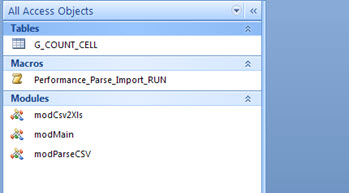
Final Table - PERF_G_CELL
Let’s start from where we left off in the last tutorial, with the GSM counters of our Netwrok in a table (‘G_COUNT_CELL’).
The first thing to do is create our first table, containing data with indicators per cell (‘PERF_G_CELL’). We can create this table the way we create any table - by using the Access interface, but it is easier to create it from a query that already has proper names and field correspondent to what it should contain - and thus use the trick of changing the query structure from ‘Select’ to type ‘Create Table’.
But first we create a simple select query, applying metrics, and getting the indicators data.
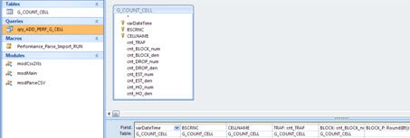
Here there is no secret, just do the math.
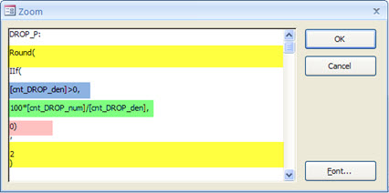
Only two observations. When we calculate a percentage value (’_P’), we must ensure that the denominator is not equal to zero. In this case, we use an ‘IF’ - in the case of Access function “IIF”. If the value compared (in blue in the example) is greater than zero, do the calculations (in green in the example), including multiplying by 100. Otherwise - value equal to zero, we assign the value zero also for the percentage (in pink in the example).
And also round off Indicator to 2 decimal places - enough for our analysis.
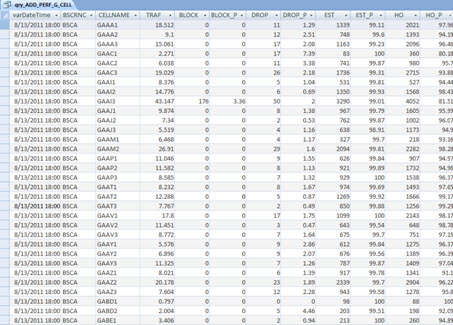
Running the query, we see our data is as expected.
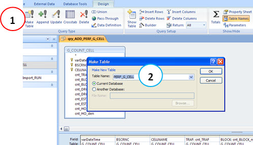
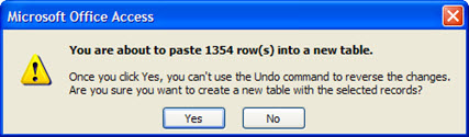
And now, to finally create the table, select the option ‘Make Table’ (1), and then enter the name of the new table ‘PERF_G_CELL’ (2).
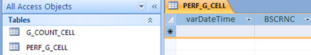
Turn this check and see that the new table is created.
Right. But our goal was simply to create the table structure. The data will be accumulated in the process: after counters data be imported into the table ‘G_COUNT_CELL’, Indicators based on its information should be accumulated at the corresponding table ‘PERF_G_CELL’.
Then delete all data from it.
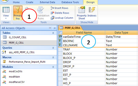
And for the same reasons that we explain to the counters table, we’ll create Primary Keys (1) for the fields that identify unique records in this table (2).
There, the table is ready to receive data in a process driven by macro and VBA code.
Add Data Query
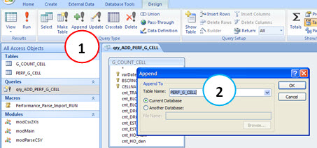
For data to be accumulated, or to be added to this table whenever the application run, we change the structure of our query to type ‘Append’ (1). Thus, whenever we execute this query, it will add its data to the specified table (2).
Now, just need add a line to the VBA code, to run this query right after importing the counters!
Table of Counters
The important information, which is necessary, is given by the indicators. That is, we don’t need to ‘also’ keep the table with the accumulated counters.
So from now on, we will not accumulate more counters - no need for it. Again, we insert a line in the code so that the data in this table are erased whenever the application run.
Final Table - PERF_G_BSCRNC
In addition to the first basic table with data per cell, we say that is important to store such data in ‘sub’ tables.
This is because these other tables contain data that are often sought for our future reports.
Then, to create a query that groups the data by BSC / RNC, create a new query. But now delete the ‘CELNAME’ field. Continue grouping the data, and make adjustments in the calculations.
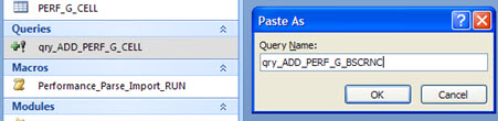
To do this simply copy and paste our previous query with the name ‘qry_ADD_PERF_G_BSCRNC’.
But we also need to create a new table to contain data.
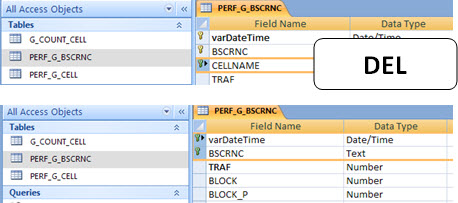
We can do just as we did earlier, but our table is already created for ‘CELL’, and the fields are the same - with the exception of ‘CELLNAME’, so we can simply copy and paste that table, saving it as a new table ‘PERF_G_BSCRNC’. Then, in its structure, we remove the extra field (‘CELLNAME’). Remember to return the remaining fields as Primary Key, because when you remove one, all others lose this attribute.
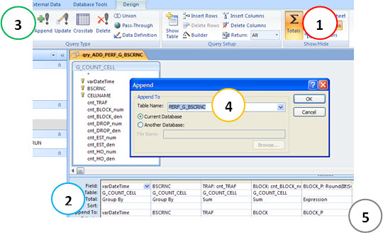
Now, in the structure of our newly created query, make the necessary adjustments. Select ‘Totals’ (1) and adjust the calculated fields in the ‘Total’ row (2). Click on ‘Append’ (3) and change the table name where the data will be added to ‘PERF_G_BSCRNC’ (4). Note that the line ‘Append’ already choose the fields of the table corresponding to the same query fields (5).
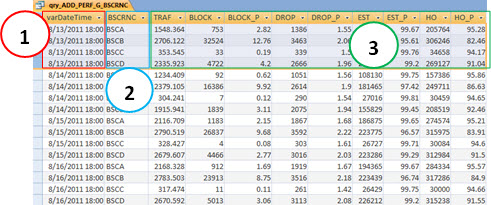
To check the data, you can temporarily run this query in selection mode/type. Here we now have the data for each period (1) grouped by BSC / RNC (2), with their calculated values as expected (3).
Final Table - PERF_G_NET
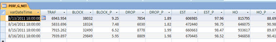
Our final table today brings together the data for the system. For each time, we have a general summary, in table ‘PERF_G_NET’.
The procedure is exactly what we did for table ‘PERF_G_BSCRNC’ - but now also remove the ‘BSCRNC’. Hint: it’s easier to copy create the second query, since it is already has adjusted calculations.
In the end, we expect the table.
Once you have created queries that add data in the corresponding tables, we need only adjust a few lines of code to perform this appropriate action.
VBA Code
Since you’re already used to, all our supplied code (Hunter Donators) is always commented. This makes the explanation again here redundant, extensive and unnecessary.
IMPORTANT: The full code, including lines with comments, is still under 100 lines! Anyway, if you find any problems or have any questions on any procedure, please contact us by posting your question in the forum.
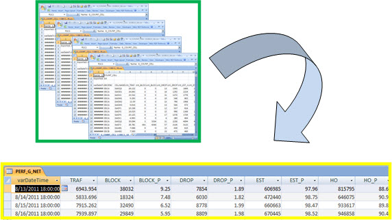
Result
As expected, the result.
Again, we don’t see big advantages in a module like this: A few simple tables with the Performance Indicators?
The only thing we can say right now: wait and you’ll see what can be done with them!
And as always: practice to learn. In addition to being extremely simple to adapt for your own scenario, you can even create new modules in the future - whatever your need and your imagination like. And of course, always count on our help.
Good, that’s it for today. We hope you enjoyed, we always try to ‘translate’ the Telecom World in a simple and easy way to understand.
And get ready for new tutorials!
Conclusion
We have seen how to create another customized application using Microsoft Access, continuing the processing of counters into Standardized KPI (Indicators) Tables.
We store the data in basic tables with granularity for System or Entire Network (NET), BSC/RNC (BSCRNC) and Cell (CELL).
Very soon we’ll use this data in a more constant way, and its importance or necessity will be perceived in practice.
Thank you for visiting and we hope that the information presented continue to serve as a starting point for your solutions and macros.
In particular, we thank You telecomHall Donator. The tutorial files was already sent, please check. If you have had a problem upon receipt, please inform.
New tutorials are ready, and will be published soon. It will become more complex (although explained in a simple way), so we recommend that you take all the doubts that happened during your readings.
Remember, your acquired knowledge can be your biggest difference, just depends on your will.
Download
Download Source Code: Blog_030_HunterPerformanceKPIBaseTables(Application)_NEW.zip (1.0 MB)