Introduction
After several tutorials to familiarize with the Hunter methodology, let’s continue now with more practical applications, ready to use on a daily basis.
Today we see the application responsible for creating KMZ files from text files or Microsoft Excel spreadsheets, exported from any commercial Drive Test Software.
Who knows the power of custom tools will be amazed how, with a little creativity, we have simple solutions but they leave nothing to be desired in relation to several existing commercial applications.
The application today, as we speak, is on the analysis of Drive Test. However, it involves a lot of tips and best practices you can use in your work.
Goal
Present the solution Hunter GE Module Drive Test. It is easier this time to present the purpose by showing the actual interface for the module.
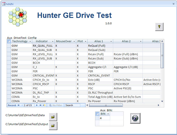
Always following the methodology presented so far, the interface allows us to interact with raw data exported from Drive Test (in TXT or XLS), and with a single click, generate the files in Google Earth, according to our desired settings .
The settings are presented in tabular form (where the data is editable). You can also adjust the BIN, which allows the generation of a lighter file (fewer points) or more detailed (all points). We will see more on this later.
We also have the option through the interface to open input directories (date - where we put the TXT / XLS) and output (Output - where the KML / KMZ are generated) of this module.
A Little Help is also available, for example where we can see that the most important fields are ‘Indicator’, ‘Mouse Over?’, And ‘Plot?’.
The field ‘Indicator’ is a reference to the desired indicator (RxLevel, ECIO, etc. …). The field ‘Mouse Over’ serves to inform you whether we want the value of each item to be displayed when you hover over it. And the ‘Plot’ tells you whether this indicator, if present in the file, should be plotted.
Fields ‘Technology’ and ‘AliasN’ are reference fields. Only serve to visualize the technology, and to know the name or names of fields expected to be plotted for each indicator.
Everything becomes a little clearer when we practice using the tool. So come and see how everything is done.
Scenario
Our scenario, as already mentioned, and we first get the data from all Drive Tests in a TXT or XLS file. From this file, plot the data on Google Earth, making all relevant treatments.
The generation of these files is an important point, but it’s not complicated. Unfortunately, we can not demonstrate here how to do for each existing software, but for sure the one you use allows you to do this.
Note: If you need help, please contact us (link on the About page) and we’ll send the step by step to your specific software.
If you do not run the data collect, but simply receives the reports of a contractor, simply ask them to send you - also - the data in TXT or XLS.
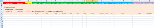
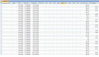
To make it easier to visualize, see the list of fields.
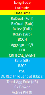
The most important fields, of course, are Latitude and Longitude, for obvious reasons.
The DateTime field is also important and desirable, although not essential. If this field is present, and contains the information of Date, it will be used in the name of the KML / KMZ, that is, you know the exact date when the Drive Test is performed.
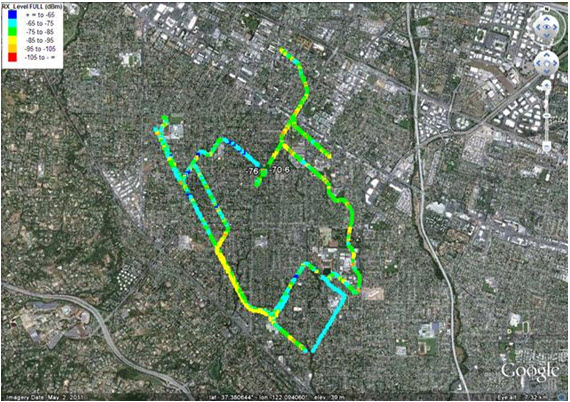
Finally we have the other fields. For example, if the file has the field ‘RxLev (Full)’, the application will plot the data from the GSM signal level. If the indicator is in the file - with the default name - and is set to be treated - the ‘Plot’ field - it will be generated. Simple as that.
For each indicator present, the data can be generated. You can have one or all of the fields depends on you exported or not. And one important thing: you do not need to process each file one by one. For example, if you put three XLS or TXT files, three KML / KMZ files will be generated, containing the corresponding indicators - present - in each file.
Note: You should note that in addition to a default name, used worldwide for each indicator, we have one or two others. Are variations, but they bring the same result.
It is easier to understand that freedom by example. If the name of one of the fields is exported ‘RxLev (Full)’ or ‘RxLev (Full) (dBm)’, whatever, the indicator will be plotted RX_LEVEL_FULL. This serves only to cases where, for some reason, you receive files with these variations. But do not worry with it and just make sure to export the data with the names of Alias1.
File Structure
The basic structure of the Hunter you know of other tutorials, and has accompanied the evolution, the directories of this module are already created.
Anyway, follow the basic structure.
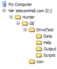
The ‘Script’ directory contains the script, which in this case is our application. The ‘Data’ directory as we speak, is where you can store all the TXT / XLS files exported. The ‘output’ directory contain all the KML / KMZ files generated. The ‘Help’ directory containing files support, such as auxiliary spreadsheets - data exported template, ranges settings for each indicator and the its legends, etc… And the ‘icon’ directory, common to all Hunter GE modules (As Performance - KPI - and Parameters) - this directory contains auxiliary files (images) that the application access to a professional presentation of data.
Without further ado, let’s talk about the application in more detail.
IMPORTANT: here we present the forms created by us to obtain the solution. This includes a series of tricks and considerations that allow us to creativity with a practical and functional outcome. Of course that can always be improvements, including some already planned and under development by us. You can even extend the application to an even higher level and suitable for your possible needs. Anyway, certainly worth learning and to understand how everything can be done.
The Application
We will first explain each of the objects (tables, queries, etc…) in theDatabase, and then show what is done through VBA code (which is only 300 lines).
Tables
Let’s start with the base table ‘DriveTest’. The data from TXT or XLS are first imported into it.
And here we have the first trick: to import files from a text file (TXT), we need to tell Access exactly what are the fields. But what if the file contains a few more fields, such as ‘Sequence No’?
Otherwise, if we were to import the text through ‘text data transfer’, we would necessarily force the file to always have exactly the same fields and format.
But when we import an XLS file into Microsoft Access, we do not need a fixed specification. And if we have a table (like ‘DriveTest’) that already has almost all the fields that could be present, we can simply to import it. The more (other) fields are blank, but our desired are imported correctly.
Thus, even though we have all the files in TXT format, the application will save each one as a temporary XLS.
Then continuing, the data of the new XLS file is transferred (via code) from the ‘data’ directory for the table, one at a time, depending on the amount of files being processed at this time.
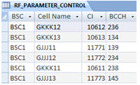
We have some auxiliary tables. One is the ‘RF_PARAMETER_CONTROL’. This table contains auxiliary data of our network, which are accessed by the application. In the example, if the field ‘CellID’ is present in the file, we can get the name of the cell in that table.
Note: RF_PARAMETERS_CONTROL is a standard table of the Hunter Parameters module, which brings together all the key parameters of the network configuration for each sector, such as BCCH, CI, BSC, among others. This table should therefore be linked to this module, and whenever it is updated, we access the data here are also updated. However, we partially replicate it here today only to facilitate.
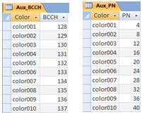
Other auxiliary tables - whose purpose we’ll understand soon - includes correspondence of values of GSM BCCH and CDMA PN with colors.
- We could use the same reasoning for UMTS PSC. However, later we will show why we’ve done a little differently for it. In this case we have the table ‘DriveTest_PSC’.
To finish the display of tables, let’s talk now of another tip.
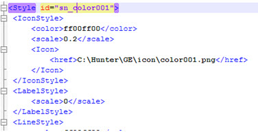
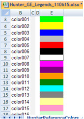
We know that Google Earth works with Styles, ie, defining a particular style with a specific name, you can assign all its features such as color and image corresponding of that style. Then for each point (Placemark) to plot, just tell it has that certain style!
And we can write all the styles in generated files in the code line by line. But when we have a lot of styles, it is worth writing the same on-the-fly ', reading the data from the auxiliary table.
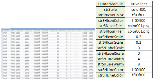
See for example, the style ‘color001’. If this style is assigned to a point on Google Earth, it will have all the properties of it - once write to the file with proper formatting!
Now that we know our tables, let’s know the queries of our application.
See that everything is pretty simple (You might not be familiar, but in time will agree it is).
Queries
We begin with the query ‘qry_Aux_GE_Styles’. Basically the data in table ‘tbl_Aux_GE_Styles’, filtered to only the styles that module ‘DriveTest’.
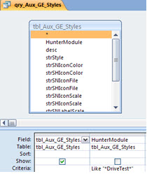
Note: You may be asking, why use a query if the table currently contains only styles, with properties for this module only. Well, actually, the table ‘tbl_Aux_GE_Styles’ in future will also reside on another database. Was replicated here only for simplicity. That is, in the future, you access this table from another database (Hunter Common), and contain the same styles to other modules. Thus, this query filters the data for this module only.
Now, almost ending , let’s talk about three most important queries.
‘Qry_DriveTest’, ‘qry_DriveTest_Coords’ and ‘qry_DriveTest_Coords_Thematic’.
The first query ‘qry_DriveTest’ is based on table ‘DriveTest’.
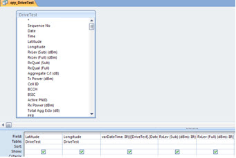
This query do some processing, but nothing too complicated. The most important thing is that the considerations made here are (calculated fields) of the alias. Returning to use the example of the variations ‘RxLev (Full)’ or ‘RxLev (Full) (dBm)’, the final field of this indicator takes into account whether the data is in one or another - as if a sum of them. Again, this is not critical, and only a workaround for a case that probably will not happens to you - will have variations of the same name field.
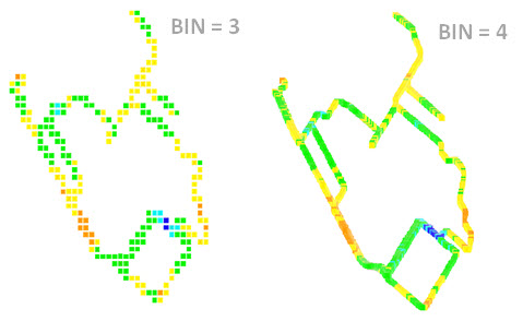
The following query - ‘qry_DriveTest_Coords’ - it’s a slight adjustment, as we said earlier, on the BIN. We use this name (bin), but actually do a far simpler - but functional. Our ‘BIN’ actually represents the number of decimal places will be ‘grouped’ for latitude and longitude data.
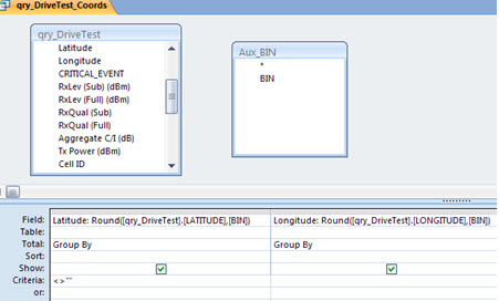
The trick here is to utilize the previous query in this query ‘qry_DriveTest’ with table ‘Aux_BIN’, which contains the BIN set. Thus, we can group (Group By) Latitude and Longitude data, decimal rounded to BIN.
And all other fields should be calculated as the mean (average). This simple procedure provides us with different plots - with more or fewer points. However, you will realize that for a visualization macro, a plot with a lower BIN may be sufficient. The gain here? Performance: fewer points = much lighter and faster to analyze the data.
You can generate such plots with lower BIN for very large DriveTests (many points), and only use higher BIN to get details in specific situations.
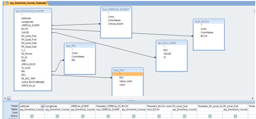
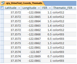
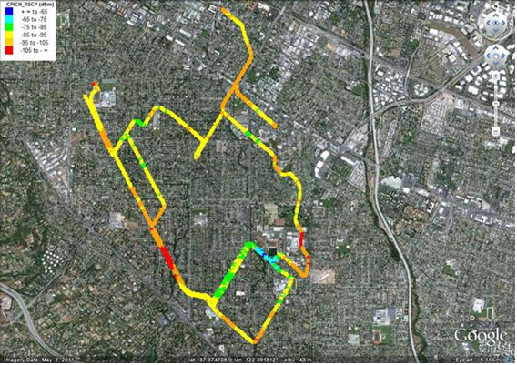
And finally, query ‘qry_DriveTest_Coords_Thematic’. In this query, we create a new calculated field for each indicator, with the style name to be assigned to that point, for each indicator.
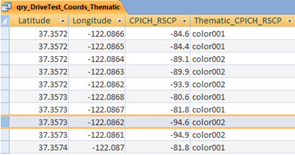
For example at the point of Latitude / Longitude 37.3573/-122.0862, the RSCP was -94.6 dBm, and we assign the style theme ‘color002’. But how we do it?
Not too tricky - although it may seem when seeing the structure of the query.
We have basically two cases.
The first, for individual values. In this case, simply tie the previous query ‘qry_DriveTest_Coords’ - that our data is already nearing completion and the estimated BIN - all queries with their corresponding auxiliary styles.
It is easier with the Aux_BCCH example, for GSM. For each BCCH of our query ‘qry_DriveTest_Coords’, when there is a corresponding value in the ‘BCCH’ table ‘Aux_BCCH’, get style (Color) that has put pre-defined in this table!
And the second theming, for ranges of values. For this, we use a calculated field for each indicator. We use the IIF - the same as Excel.
Here’s an example Thematic_FER for example:
Thematic_FER:
IIf ([ERF] <= 1), “color003”
IIf (([Fe]> 1 And [ERF] <= 2), “color012”
And so on.
Well, that explains the operation of the application’s point of view of data processing.
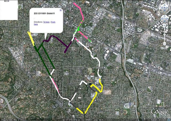
Let’s just talk now about the issue of UMTS PSC: Why we did different as GSM BCCH and CDMA PN?
In fact, we could use the same solution that we now show for BCCH and PN.
But: imagine a network with numerous PSC. And suppose you create an auxiliary table for each value of PSC. Also, you set a color for each. The problem is that the range of distinct colors are shallow (eg Hunter, have 56 defined, and even then with great difficulty).
![]()
But in a Drive Test you do not have ALL of your network PSC!
For example, if you have say 20 PSC, you can use a different color for each of them: and then, you see most distinctly the coverage area of each sector.
But how?
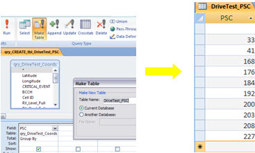
Here, a trick. First, from the PSC DriveTest present in the table, we generate a table axuliar ‘DriveTest_PSC’. For this, we have a query ‘Create Table’, which we call ‘qry_CREATE_tbl_DriveTest_PSC’, and when it is executed, our table is created.
That’s half the battle. Now we need some way to assign styles (colors) sequentially, guaranteed and to distinguish sectors. And for that, and concluding on queris study for today, we create a ‘rank’ query in Access.
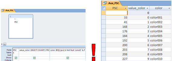
This query is very simple, and we’ll explain it later in detail in a brief tutorial in the tips section. This type of query is very powerful, and used in several other modules of the Hunter, mainly Performance / KPI.
For now, just understand that the query generates a sequence number to each row of the query. And simply use that number (value) to fill our style - color001, color002, and so on.
So, it ensure that the PSC will be as distinct as possible. (As we have 56 colors in the Hunter, only began to have reps from rank 56 - and then the match - sectors close to the same value - is also much harder to occur!)
Images Auxiliary
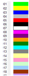
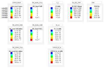
In previous tutorials, you’ve learned to use images to get the plot for each point with the desired characteristics (color, icon, etc.). And also how to display the legend of each file.
It is important to maintain a standard spreadsheet, with the definition of each color, and their respective value and style.
For each of these 56 color images were created, the images are available in the ‘icon’ directory, and accessed when needed.
Likewise, for each module, the legends can be created and / or modified.
Code VBA
In telecomHall, we write tutorials using Microsoft Word. And at this point, we realize we’re already on page 14! It’s too big for any web tutorial.
If we were to go through the code for this module, though it is not so extensive, the tutorial would be extremely long and tiring.
Anyway, we have virtually nothing very new or different from the codes shown in other tutorials.
If you wish, contact (About page) and ask for help routines that you want to be explained in a later tutorial.
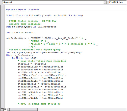
To show that nothing is new, see for example how to write the styles on-the-fly '.
We create the function ‘PrintGEStyles’. This function takes as arguments the opened file (h) and the directory where the images are (strIconDir). Next we define our SQL table (strStylesQuery) to work with the Recordset for this string SQL (rs_StylesQuery). We read the values to variables, and then write (Print) in the file.
And as always: the code should be fully discussed. Always.
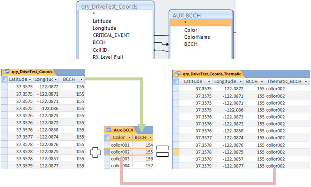
Results
The result of this module is as expected. Plots for different indicators in Google Earth KML / KMZ!
Here are some examples.
Well, that’s it for today.
Conclusion
We have seen how to create a custom application using Microsoft Access to plot indicators of Drive Test in Google Earth KML / KMZ format.
The application is comprehensive and functional, allows the professional to use and get better results when analysing and/or presenting data to others.
Thank you for visiting and we hope that the information presented can serve as a starting point for your own solutions and macros.
In particular, we thank the Donators of telecomHall. The tutorial files that have already been sent (donators only), please check. If you have had a problem upon receipt, please inform.
Download
Download Source Code: Blog_026_HunterGEDriveTest(Application).zip (2.1 MB)