Introduction
The reach area of each cell of the network directly affects the efficiency of the system in terms of Quality, Capacity and Coverage.
Therefore it is essential that each one be perfectly adjusted. These adjustments include changes to the configuration parameters (eg, for load balancing), and also adjustment of physical parameters.
In the latter case, the adjustment of tilts and azimuths (and sometimes height) of the antennas is a key factor in achieving the best possible results.
The opposite is also true: if the tilts and azimuths are not properly adjusted, the task of improving the network becomes virtually impossible. If the physical settings are not fine, no configuration parameters to improve the network.
The problem is that this type of analysis is not simple, because it usually involves complicated analysis. It is necessary to evaluate, for the same cell, different existing technologies (2G, 3G, 4G) with possible different layers (frequency and / or carriers).
Existing tools for this type of task are pretty “heavy” (prediction tools with complex calculations to estimate signal coverage, and almost never deal with “all” the layers together). Moreover, they require a lot of time for loading the data, and setting many details. Details such that not all professionals are always familiar.
Thus, a tool that allows us a quick analysis of this scenario can bring substantial gains in improving the Quality, Capacity and Coverage in general, improving satisfaction of users.
Moreover, a network poorly adjusted in terms of azimuths and tilts can lead to errors in planning, which may require new cells (many of which may not be necessary with a proper design of the radiating system).
And to solve this problem, we developed another application, an additional Hunter module to help us in this quick check.
Let’s know the details of this application.
Goal
Present the main functions of the module “Hunter GE CoverTune”.
As always, the module is a complete application, including data from a fictitious network. Thus, HUNTER Users can use it as is (simply adjusting the data from their actual network), but also making customizations / enhancements in the same according to their needs.
User Interface
The main interface is as always very simple - the main commands you need, and again, allowing any type of customization.
When you receive the source files, you can extract them and build the structure shown below.
Note: remember that all of the dozens of modules that you’ve received till today follow the same structure, and you’ve extracted all the local folder to "C:". So, when you extract the files of this module today, your structure will be greater than shown below.
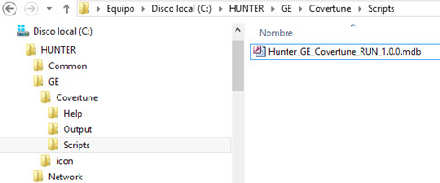
The main interface of the module is now accessed by opening the “Hunter_GE_Covertune_RUN_1.0.0.mdb” file (located in the Scripts directory of this module).
Increasingly we will focus on the “use” of the modules. If you have any questions on customization of this module, please use our Forum here.
Using the Module
As already mentioned, this module allows the rapid analysis of coverage of each network cell.
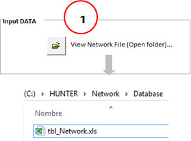
The main input that you must have, of course, is a simple table with the network data (latitude, longitude, antennas, azimuths, etc…). This is a table that follows Hunter standardization, and is in "C:\HUNTER\Network\Database" directory. In today’s example, we have a link to that table in Access from Excel, but remember that you can also get data from any other source (simply linking that table), for example, a network table in another Microsoft Access file.
And you can easily access this file through the button (1) that opens the directory where it is located.
When you open this file, you will see the data from your network (in this case, our fictitious sample data).
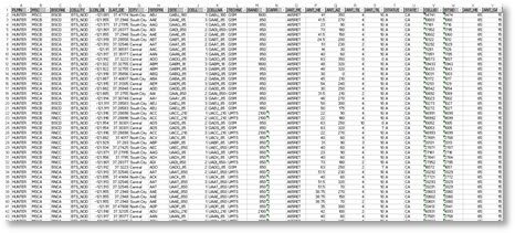
Changing the data in this table, the results are automatically updated (running the macro again).
All other entries are just adjustments, such as those that define the colors and other attributes of polygons and other objects from Google Earth that will be created. And you can also access this file directly through the interface of this module: “Cell Type Map” (1) tab.
The “Cell Type Map” is needed as a way to identify the different layers and how each must be customized (colors, etc…).
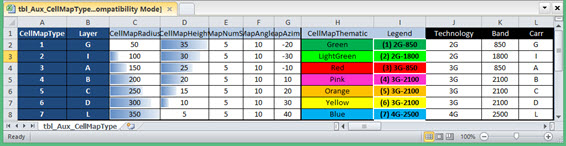
This table setting is common to all other modules that need the information contained herein. For example, when you create a file with all your cells, or when plotting Parameters or KPIs in Google Earth, it is from here all modules get information for each layer, etc…
In today’s case specifically, we will not use all the data. Basically we need here only the layer information (“CellMapType” field) and its attributes.
For example, if the network cell table is CellMapType = 1 then will have a Green color. If CellMapType = 4, then the color is Pink. And so on.
The “Technology”, “Band” and “Carr” are auxiliary fields, and allow you to easily set the attributes of the layers, based on these entries.
Tip: Also, even if you do not have “CellMapType” field in your table the network - is usually what happens, and it is also the case in this example today - you can create a query using this table and the network table, thus generating a query with the “new” network table - which will now have the “CellMapType” field according to your choices.
But everything is easier practicing, and we will do so shortly.
Let’s just finish commenting on some other items from the main interface.
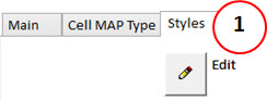
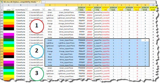
One is the “Styles” (1), another Excel spreadsheet that you are already familiar, where we define “styles” (colors, line sizes, etc.) and which will later be associated to the corresponding cells.
Here there is a little explanation.
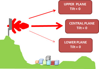
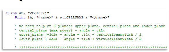
Today we are not specifically plotting the “coverage” of the cell, but the “coverage” of “Central”, “Upper” and “Lower” planes of the antenna radiation pattern.
The figure below helps us to better understand. For the same tilt (eg, zero), we have three different planes, according to the vertical antenna bandwidth.
An excerpt from the source code shows the formulas used in GIS calculations.
And it is these same plans that are also represented in attributes. For example, in the screenshot below we can define different attributes for “Central Plane” (1) “Upper Plane” (2) “Lower Plane” (3).
Note: once again we remind you that these are “possible” customizations, however you can use all the settings the way they are, and will have a very good result for your analysis.
Let’s finish the description of the items of the main interface.
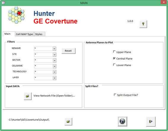
Returning to the “Main” tab, we see the possible filters (1). With them you have the flexibility to generate files according to your choice (for NENAME, cellName, SITENAME, etc … ).
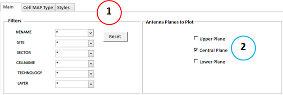
And with “checkbox” (2) we can choose the plans (only one - as in our case the main “Central Plane”; two of them; or all) we want to plot.
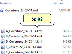
Finally, one other feature of this module is the ability (1) to split the output file into multiple files.
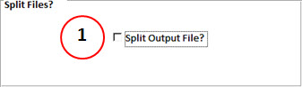
This is especially useful if you have a very large network (over 3,000 cells), and want to generate all at once. If you select this “checkbox”, a file will be generated for each group with the first letter of the site data.
Explaining better: assuming you have a “ACX” site and another “DDF” on your network. The cells from site “ACX” will be plotted on the file that starts with “A_”, and the cells from site “DDF” will be plotted on the file that starts with “D_”.
Good. Enough description for today. We’ll now see the results, since the best way to learn is by practicing.
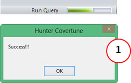
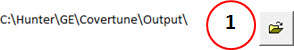
Simply open the program, and click the “Run” icon. After a few seconds, a confirmation successful screen appears (1), stating that the files are already available in the “C:\HUNTER\GE\Covertune\Output\” directory.
You can easily open these files: Click the corresponding button (1) to open that directory.
Opening this file, you already have everything ready to analyze your network.
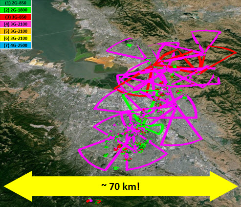
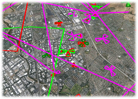
The overview already indicates several problems. Numerous cells with the central plane at a distance of several kilometers (larger polygons in the figure).
Clicking on any of these cases, for example, “UABC_2100-1” cell, we have identified the reason for this anomaly: this cell has Tilt Total (Electrical and Mechanical) equal to Zero!
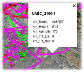
This is a quick analysis of what we can do in any network, and that can help us greatly in identifying similar cases (very low tilts, or coverage beyond what should be).
Note: In this particular case, a cell in the network edge, this situation is not as “critical”. But in other cases in central cells which should have the coverage more “contained”, it is probably causing problems.
Nevertheless, let’s take that same cell to another type of analysis.
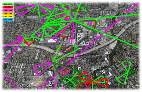
According to the sample data, this sector has 2 cells: a 2G-GSM (GABC_850-1 Green in the Figure) and other 3G-UMTS (UABC_2100-1 Pink in the Figure).
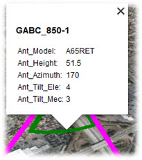
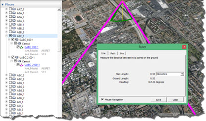
We see in the figure above the central plane (determined by full tilt and vertical antenna bandwidth) 2G cell is about 500 meters, while in the same sector, 3G cell has its central plane at several miles! It is not difficult to understand the problem, isn’t it?
That is, in a very simple way, we saw a case of a critical situation (not desired) as shown in the figure below.
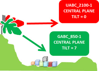
In these cases there’s no parameter optimization that solve the problems caused by this situation. Be among 2G and 3G, and also between different 3G carrier, and even 4G!
Nor is it necessary to say (although we have said before) that such cases are even more critical in denser regions. In the figure below, identify areas with potential problems (larger radius overlapping several smaller radius).
And we can also use the results to a good prediction* approximation. Naturally, the results and defined actions should always be confirmed (via prediction tools). But in practice, the initial simple adjustments of the discordant cases brings an impressive result for the entire network - Capacity, Quality and Coverage, as we talk at the beginning of this tutorial.
Remember that we are dealing with fictitious data. But do not be surprised if you find cases very similar in your network - and show the suggestions to your boss!
And no need to thank us, you’ve done it, when you made your donation. This motivates us to develop new modules that can always bring simple and effective and results to the overall improvement of your system.
Very soon we’ll make available other tutorials: eg “Hunter Covertune XL” - a fantastic macro in Excel that allows you to identify unbalance problems (among others) using the table that you already have with the network data.
Another tutorial that is also nearing completion is the “Hunter GE Mapcell” - we’re converting the application from MapInfo / Mapbasic:
in an easy to use Google Earth application, and with many more features.
And again, be sure to continue to participate in other sections of the website - especially the courses section, where we are publishing a series of tutorials explaining in a simple way (as always) complex LTE Concepts.
Conclusion
Today we saw a new Hunter module that allows to do a very fast analysis, but also very efficient on the coverage of all Network cells.
From the results (generated files) this kind of complex analysis becomes trivial. Identify problems and trigger actions becomes incredibly simple, and while quite significant in terms of improvements in virtually all aspects of the network (capacity, coverage and quality). And of course, gains on investments: a well optimized network will require new cells only when really needed!
Again thank you for visiting. Keep participating and being part of this world community that every day grows a little more!
Until the next tutorial.
Download
Download Source Code: Blog_040_Hunter_Google_Earth_CoverTune_(Application).zip (698.2 KB)