Introduction
We’re starting a new sequence of Hunter Tool tutorial. In today’s tutorial we will see the module ‘Hunter GE Propagation Analyzer’, which deals with Performance counters collected data and plots them in Google Earth.
That way we can perform different types of analysis, as shown in detail in tutorial:
Analyzing Coverage with Propagation Delay - PD and Timing Advance - TA (GSM-WCDMA-LTE)
Its reading is highly recommended before proceeding.
Here we go for the tutorial.
Goal
Briefly present the module ‘Hunter GE Propagation Analyzer’, serving as the basis for initial use and/or modifications on it.
User Interface
The interface of the Hunter modules virtually does not change: it’s pretty simple, allowing you to make any customizations that you find convenient. It’s always just a starting point - although it can be used as is.
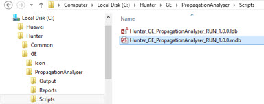
Below is the main interface of today module, that appears when you open the file ‘Hunter_GE_PropagationAnalyser_RUN_1.0.0.mdb’ in ‘Scripts’ folder of this module.
Note: After practicing the ‘installation’ (actually file extraction) of the modules in dozens of previous Hunter tutorials, you should already be familiar with this task. Even so, if you encounter any problem in playing what we have shown here, please contact us.
Using the module
Let’s cut to the chase and show you briefly how this module works. More details you can find using the files provided - tables, queries, and macros, all with VBA code commented.
This module handles ‘Propagation Delay’ data, which must be in the Hunter format, as reported in the tutorial with an explanation of ‘Propagation Delay’, which we recommend at the beginning (again: If you haven’t read it, we recommend you to do this).
In this tutorial, the sample data are stored in an Access table, but as always, they might be in another format, such as an Excel worksheet. If you want to use another form, simply make the corresponding changes - also must be common to you that processing of data from different sources. But if you have any questions, please contact.
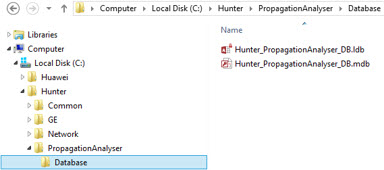
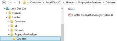
So, our raw data (table) are available in the file ‘Hunter_PropagationAnalyser_DB’ in the ‘Database’ folder.
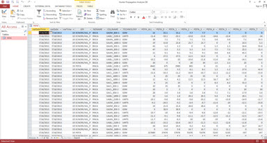
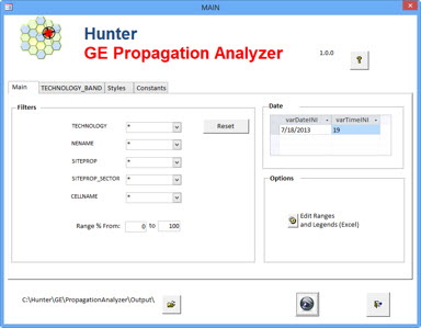
Back to the main screen of the application that will handle this data (which are linked to), let’s talk about only of what is new in this module. Note: the data are in ‘PDTA’ table linked from ‘Hunter_PropagationAnalyzer_DB’ database.
![]()
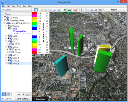
As always, to plot the data, just click on the button with the icon of Google Earth.
![]()
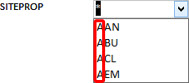
The only thing new here today are the filters that can be applied, allowing you for example filter only a Technology (1), only a BSC/RNC (2), only a SITEPROP (3), a SITEPROP_SECTOR (4) or more specifically, only one cell (5).
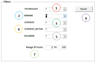
The ‘Reset’ button (6) returns the original values.
And the ‘range’ (7) allows you to make a specific analysis, only for a certain range of contribution. For example, if you type 50 to 100% then only items that meet this criteria are plotted.
Adjusting Ranges and Legends
By clicking the ‘Edit Ranges and Legends’ (1), you can configure the options of ranges and legends.
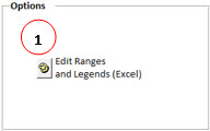
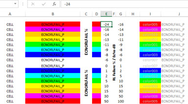
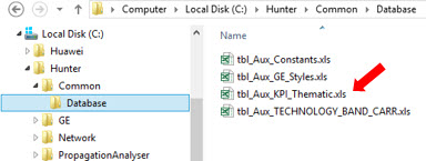
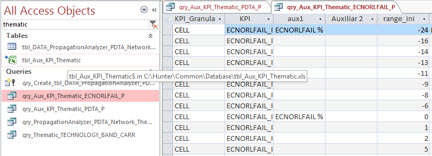
Edits are made - and are stored in Excel file ‘tbl_Aux_KPI_Thematic.xls’, the same KPI configuration file of all Hunter Modules.
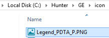
Note: whenever you make a change in your ranges, values or colors, remember to also update the legend file ‘Legend_PDTA_P.png’, so that it corresponds to what is in Excel.
In our Access application, the queries ‘qry_Aux_KPI_Thematic_ECNORLFAIL_P’ and ‘qry_Aux_KPI_Thematic_PDTA_P’ seek these data via linked table ‘tbl_Aux_KPI_Thematic’, providing the data configured for these ranges to be handled by the application.
Dividing the output into multiple files
And as you might imagine, if you process all your network cells (all cells of all GSM BSCs, and all cells of all UMTS RNCs) you may end up generating a very large file.
So how can we split these output data?
Some people have some ideas or suggestions. For example, generate a file for each BSC and each RNC. This way it even works, but is not recommended. Let’s see why.
Imagine you have a cell - ‘GSM-AAN1’, and in the same place a cell ‘UMTS-AAN1’. If we divide by BSC/RNC, when we analyze the site spreads ‘AAN’ (propagation to both GSM and UMTS technologies), how does this work?
Yes, we’d have to open 2 files - one that was generated with data from the BSC (containing GSM-AAN1), and another that was generated with data from the RNC (containing UMTS-AAN1).
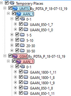
The best solution we found to this problem - at least so far - was to use the first letter of ‘SITEPROP’, or location of the site, to make this Division.
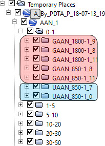
And for that, we have an auxiliary table, with letters (from A to Z). If we have a ‘SITEPROP’ starting with ‘A’, all your cells will be plotted in the file ‘A_.kml’. If you start with ‘B’, the data will be in the file 'B_.kml’, and so on.
To do this in your application, we create an auxiliary table ‘tbl_AUX_CHAR’, with the initial characters.
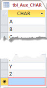
The application scans this table, and creates a file for each one of the letters that exist in this table - provided of course that they are in the data table.
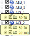
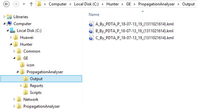
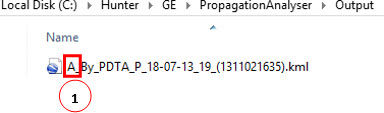
In today example we only have 4 ‘SITEPROP’, and all starts with ‘A’.
Running the program, we have the result: a file begins with the letter ‘A’ (1) - with all our cells.
Another interesting trick, yet related to the nomenclature of output files, is about processing time, or when it was created.
This is also necessary because we can do an analysis with some filter, and some time later, another analysis, with other filters. If the only form of differentiation was the first letter, the file would be overwritten.
Inserting processing hours also in the file name (2) they are never overwritten. (The processing time is entered in the form ‘aammddhhmm’).
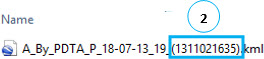
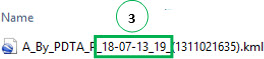
Also check that the file name contains the date and time of the data (3) present in the original table. This avoids any confusion about the date and time that these data refer.
These are the main news of this module.
We recommend that you run the sample files, and find out more details of the operation, and thus make your improvements, if desired.
All the code is open (without passwords) and commented.
If you have any questions, or would like to suggest some improvement, feel free to share with the group.
Note that this tutorial is not a complete step-by-step covering all possible points. But as an application ready to use, and with sample data to test, we believe to be an excellent starting point, even for immediate use.
Conclusion
We saw today the Hunter module responsible for plotting ‘Propagation Delay’ data in Google Earth, another excellent type of analysis that should be explored, as we have seen in detail in tutorial:
Analyzing Coverage with Propagation Delay - PD and Timing Advance - TA (GSM-WCDMA-LTE)
We appreciate your visit, and once again we would like to thank everyone, especially the Hunter Users that make this project every day more interesting. Share your ideas, and feel free to make suggestions or request new modules.
Until the next tutorial.
Download
Download Source Code: Blog_039_Hunter_Google_Earth_Propagation_Analyzer_(Application).zip (941.0 KB)