Hunter 027 - GE Network (Application)

[admin]

Introduction

With the plot of the network information (sites and cells) in a geo-referenced way, we can greatly benefit from an easier and more intuitive visualization of it, and it also helps identify problems such as misdirected cells (azimuths).

And when these data comes geo-referenced to Google Earth, it gets even better, because we can also have an intuitive understanding of the actual coverage area of the serves cells.

Today we will see a complete, customized and easily extensible application, responsible for creating KMZ files - Google Earth format - with this data.

The great advantage of this custom tool is not only that the user can quickly generate for his current network, but also can modify or add features according to his needs - which is not possible in similar commercial applications - that do not provide its source code.

Goal

Present the solution of the Hunter GE Network Module.

Note 1: This module is currently complete, but we still have many improvements that will be published later. This is because we need to take some time for donators of telecomHall to practice, read the received code, learn! These improvements may also be suggested by them, and will be included with time.

Note 2: If you are not an donator, but is interested in developing similar application, this step by step, like all step by step for all Hunter modules, you will find here an excellent starting point, with tips that you can not find elsewhere.

Note 3: soon soon, the next tutorial, we are engaging significantly in the world of Performance Indicators. Ready applications and very interesting - delta KPI, rank, full reports by e-mail, among other important algorithms very efficient and you will learn here. So, get ready for what comes around, but be sure to read any tutorials before, and mainly becoming familiar with these tools to improve our works.

Without further comment, let’s start showing the basic interface of this module.

Note: Please note that we try to keep a clean and simplified interface. This is because our application is an SDK - Development Starter Kit - and it makes no sense to be more advanced than this, at least for now.

This interface interacts with the data of our table that has Network Data (module Hunter Network).

Note: In order to facilitate the demonstration, today the table is physically in this file - not recommended. The network data - table - should be in a single location (in case the Hunter Network module). Thus other modules, not only the GE Network can access the updated and accurate data.

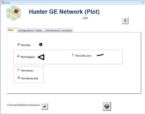
Settings are now displayed in different tabs.

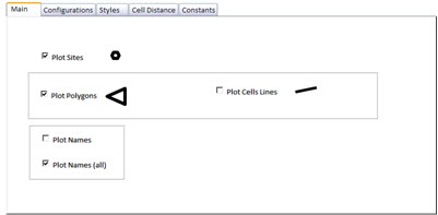
In the first tab (Main) we have simple options of choice. Here you can of course choose the cells to be created as polygons, lines, or both.

The other tabs do not need to be changed always. They contain information from the network, to inform the tool the network settings exist and whether they should be plotted.

For example in Configurations tab, we inform the technologies, bands and core elements of the network (group) like GSM BSC and UMTS RNC.

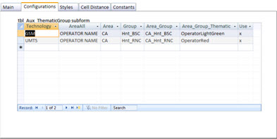
Note that in our example we have two network technologies (GSM 900 and UMTS 2100), with their BSC - ‘Hnt_BSC’ and RNC ‘Hnt_RNC’. The Area field represents a geographical area, usually an entire state with several BSC / RNC 's. The ‘Use’ field, indicates whether the corresponding data record must be plotted. This allows you to generate such a file only for GSM (and not UMTS) simply unchecking correspondign line.

And the field ‘Area_Group_Thematic’ is the most important. Here you choose the color applied to each group / technology. Later we’ll explain this better, but for example, if the value is as ‘OperatorRed’, data will be ‘red’.

In the Styles tab, we have a table with information on all the attributes of each style. For example when we draw a red section (OperatorRed), all required information are sought here, as the KML code for color.

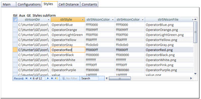
Note: you will notice that this table does not need much change. Just choose any one of these styles to apply - as we did on the previous tab, where we define cells of the UMTS RNC ‘Hnt_RNC’ as red.

Also, if you need to batch update, we have a simpler option - this table is in Excel format, which can be modified and pasted back here.

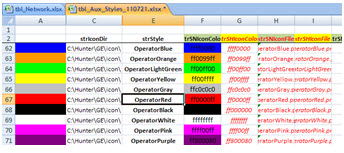
If you want to change the data in this table using Excel, you need to change just a few, the other info comes from formulas (red fields). Anyway, you have total freedom to do as you wish.

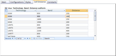
The next tab contains the information of ‘length’ of the cell. This length is defined in meters, and can be amended in accordance with their existing technologies and bands. See for example we define GSM 900 cells with 300 meters.

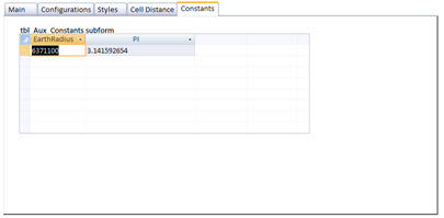
Finally, we have a last tab, with information on constants that are accessed by the tool and used in the calculations of the cells.

As with other modules, we have the option to directly open the location (directory) where the files are generated. This further streamlines the interaction.

A little help can be accessed through ‘Help’, with the help of the main information module.

And finally the main button with Google Earth symbol, which generates the data.

Do not worry if it seems ‘much’ information. Everything becomes clearer when we practice using the tool. So come on, and now do with a bit more detail the objects (tables, queries, etc…) of Database.

Scenario

Our scenario is now well defined - from a single table with the data - technology, coordinates, bearings, etc… - Generate the data in Google Earth, making all the necessary treatments.

Of course, that for the data to be plotted correctly, some fields are required. To facilitate adpatation for your network, it already is a functional application, with our dummy data, and you still receive the Hunter Network table in Excel format. Remember that this table will contain increasingly more important field for our evolution in near future.

For convenience, if you have any difficulties, first practice with the tool with the data already available (dummy data of Hunter Network).

Then, to generate the data from your network without any problems, just put the data in the same format of the worksheet you received. Then paste the data in the module table.

Note: once again reminding - in fact, you must have this data in a table of the Network module, and bind it. But for example, and practice, you can use the table physically here in this sample. Believe me, over time, you will see that this is a good practice, even if they might still find it a bit tricky - but it is not.

IMPORTANT: But I need to follow this nomenclature? The answer is no. To practice, we recommend that you follow, even to avoid problems with unnecessary errors. But you can have your table for your network in a different format, especially the names of the fields. Soon we will see to circumvent this problem easily - and you do not need to change anything in your existing data.

File Structure

The basic structure of the Hunter you know of other tutorials, and has accompanied the evolution, the directories of this module are already created.

Anyway, follow the basic structure.

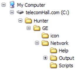
The ‘Script’ directory contains the script, which in this case is our application. The ‘output’ directory contains all the KML / KMZ generated files. The ‘Help’ directory contains support files, such as auxiliary spreadsheets. And the ‘icon’ directory, common to all Hunter GE modules (As Performance / KPI and Parameters) this directory contains auxiliary files that the application access to a professional presentation of data.

Now let’s talk in more detail the application.

IMPORTANT: presented here is the way created by us to obtain this solution. This includes a series of tricks and considerations, which allows us with creativity have a practical and functional outcome. Of course that can always be improvements, including some already planned and under development. You can even extend the application to an even higher level and suitable for your possible needs. Anyway, certainly worth learning, at least to understand how everything can be done.

The Application

The entire application is done in Access with VBA. Let’s see important details about the development.

Database objects (Tables, Queries, Macros and Forms)

Let’s start talking about the auxiliary tables, explaining its purpose.

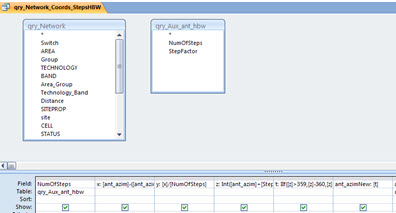
We start the table ‘tbl_Aux_AntHBW’, and its corresponding query ‘qry_Aux_AntHBW’. The purpose of this query (the table has all data, the query are filtered data which is accessed by the code) is to provide steps to aid in the calculation of polygons. Represents the number of points we have in the circumference of the semi-circle of the polygon in the cell.

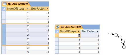
That’s right, this is already a first trick we use here. Every circle in the plot is really just a series of connected lines (points). The more points, more accurate is the circle. But you will see that a ‘4’ step - which is what we use - is more than enough. (You can practice changing the criterion of this query, and seeing how the polygons are generated).

Another table, ‘tbl_Aux_CheckBoxes’ also represents an interesting gimmick. This table stores the states of the checkbox on the main form.

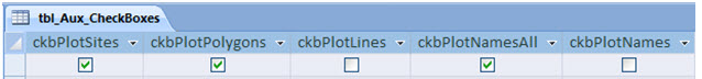
If we didn’t store these values, whenever you open the application, the figures would be standard, not the ones you used last time. Also, with all our settings stored in tables, you can run the application directly from the main macro ‘Network_GE_Plot_RUN’ - as the code reads the values that are in a table. Just to finish about macros, since we speak of them, the macro ‘Autoexec’ is responsible for opening the user interface when the application is called.

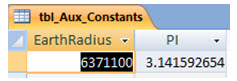
Returning to the tables, table ‘tbl_Aux_Constants’ is extremely simple and serves only to store constants that are used in the cell calculations based in azimuth and distance.

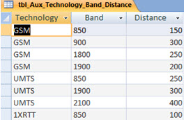
Speaking of distance, it is defined by the values of table ‘tbl_Aux_Technology_Band_Distance’ - accessed by the query ‘qry_Aux_Technology_Band_Distance’. Values are in meters, and you can change according to what you want, either by the interface, or directly in the table.

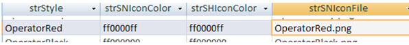
Finally, the last two tables that define the styles of each of our cells.

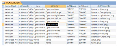
As mentioned earlier, this is where the styles are defined, and their corresponding attributes. Using the same example, if we added a Style ‘OperatorRed’, we must also add all the attributes of that style. For example, if the cell is a line, what should be its color? Red, or speaking in terms of Google Earth, ‘ff0000ff’. And so on, also for other attributes such as 'How thick is the line?.

You can update the data directly in this table, but is recommended to keep the same in an Excel spreadsheet, make changes - including the visual aid of color - and then paste it all back in this table.

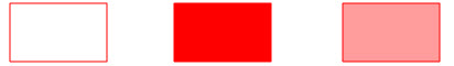
TIP: The first two characters of color ‘ff0000ff’ represents transparency. Thus, the color '000000ff 'is totally transparent (00), the color ‘ff0000ff’ is completely red, and intermediate color ‘4c0000ff’ - for example - corresponds to a 30% transparency.

Note: In the Help directory of this module, you will find a tool that helps you create your own colors and codes, including “capture” any color you want.

And the other table is the style-related ‘tbl_Aux_ThematicGroup’. This table define the field ‘Area_Group_Thematic’ with the style we want for each and Technology Group / Area.

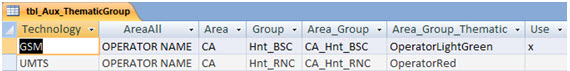
Now, a short break to explain the concept. Clusters or Groups are made for each BSC / RCN may have a different style, eg making it easier to identify the edges/borders of our network. We could simply group by BSC / RNC, but included the area that can contain multiple BSC / RNC 's. This is because some networks are spread over several states, and can thus have an appropriate grouping.

Although at first this may seem a bit complicated, is not. As mentioned before, when you practice you will see how simple and functional.

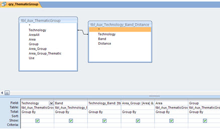
Speaking now of queries, the ‘qry_ThematicGroup’ is used to join in a query the configuration data of our network to be plotted (tbl_Aux_ ThematicGroup) with the distance data (tbl_Aux_Technology_Band_Distance).

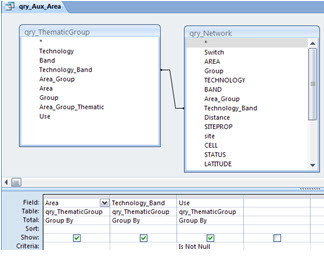
The query ‘qry_Aux_Area’ serves two purposes: to limit the processed data that are present in the archive of our network - because we can set Theme for various bands and technologies beyond what we have in a particular network - and also serves to limit the data to be plotted - the ‘Use’ field.

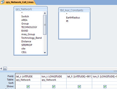
The query ‘qry_Network_Cell_Lines’ is accessed by code when we plot the data cells in forms of lines, and uses the constants for the formulas. (The formulas used have been combatants displayed in other tutorials, so there is no need to repeat here).

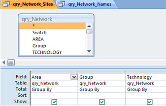
Queries ‘qry_Network_Names’ and ‘qry_Network_Sites’ are accessed by the code to respectively plot the sites and its names - when selected in the interface and / or tables.

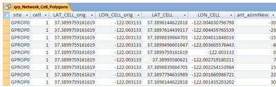
Finally, the query that accesses the code with the data to generate the polygons is the ‘qry_Network_Cell_Polygons’.

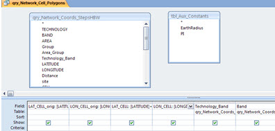
Follows the same reasoning of the query that generates the end points of each cell, but now, we have not only an end point for the cell, as in lines. Now we have several end points that define the semi-circle of the polygon in the cell.

And to achieve this, we use another ‘trick’, performed by the query. This query uses the query with our steps (qry_Network_Coords_StepsHBW), to define ‘temporary’ azimuths. These temporary bearings are used at the final query before it generates the data of polygons.

The result: for each new temporary azimuth, we have the point of latitude and longitude of the cell. These data are then processed by the VBA code, which puts them in a single line for each cell - creating our polygon.

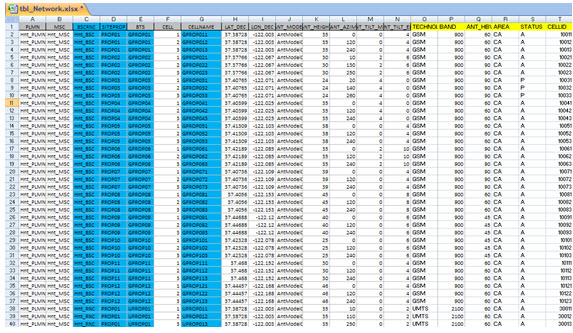
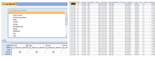
To conclude, we must now speak of the table ‘tbl_Network’. The query ‘qry_Network’, which effectively has the data we use in all other tables, has two steps (queries) before - it is not directly based on table ‘tbl_Network’.

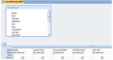
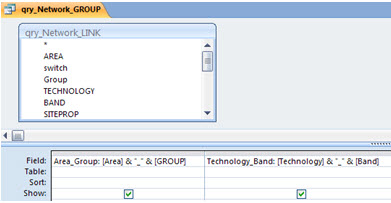
First, the query ‘qry_Network_LINK’ brings the data from our table ‘tbl_Network’, but makes a small adjustment. (Do not confuse the name LINK with the linked tables okay?). This link that this query does is adjust the names to our standard.

This is the solution for example you can use to link the data in your format / naming for application data. Note that here we use the nomenclature ‘site’ for each equipment. Only at our table, this field is named BTS. In this case, the query has a calculated field ‘site: BTS’. That is, using this query as the basis - instead of the original table - our application does not change, and neither our original data.

The idea is simple, but the gains are great. Suppose the name of our table for some reason, now switch from BTS to BTS_NodeB. Just turn on that query, and report that now ‘site: BTS_NodeB’.

And another query, this query we’ll do now, can make some other adjustments, now in relation to calculations and calculated fields. For example, here we group the fields ‘Technology_Band’ and ‘Area_Group’ - we do not have these fields that would be redundant in our original table.

Now yes, finally we create our main query ‘qry_Network’. This is the query in which all others are based, and already have all the data in the desired / expected format by the tool.

Auxiliary Images

This module does not require many auxiliary images, icons only for your carrier (network) and a Legend file.

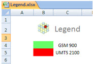
For the file (image) of the Legend, you can create it using even Windows Paintbrush. After editing, simply save it as C:\Hunter\GE\icon\Legend_Network.PNG.

Note: You also received a file Legend.xlsx. You can create your legend in Excel, and then take a PrintScreen. Then open the Paintbrush and make final edits - cutting only the desired part and saving.

For equipment files (sites), you can create small icons for your operator/network. If you prefer, create a single one with the transparent background - but rename for each style you have set and using.

Important: This icon must be small, about 30x30 pixels. Anyway, you can adjust the size according to what you want.

Note: The icon size can also be defined in the table of styles - strHIconScale and strNIconScale fields, respectively icon sizes with and without the mouse over it in time.

This trick is also used to give prominence to an cell whose mouse is over it now. strNLineWidth and strHLineWidth, in the same way that the thickness of the line - with and without mouse over.

VBA Code

Since you’re already used to, all our supplied code is always commented. This makes the explanation again here redundant, extensive and unnecessary.

If you find any problems or have any questions on any procedure, please contact us.

Result

Again, a module with the expected result: network information (sites, azimuths, etc…) are plotted so geo-referenced Google Earth.

The combinations are numerous, depending on your settings, their styles (sizes, colors, etc…), Your network!

Here are some examples for our dummy data.

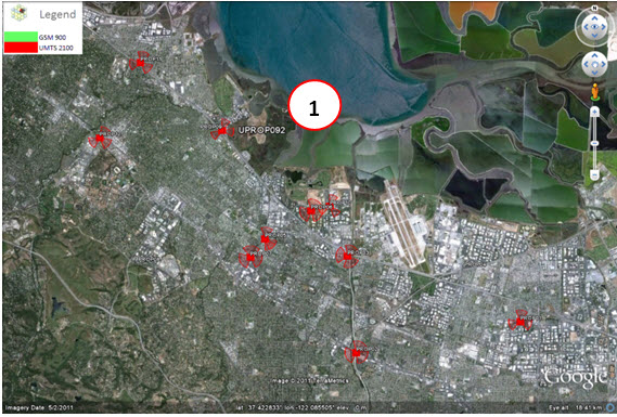
Example plot only UMTS 2100 network, with transparency. A feature common to all - when passing the mouse over a cell, its name appears (1).

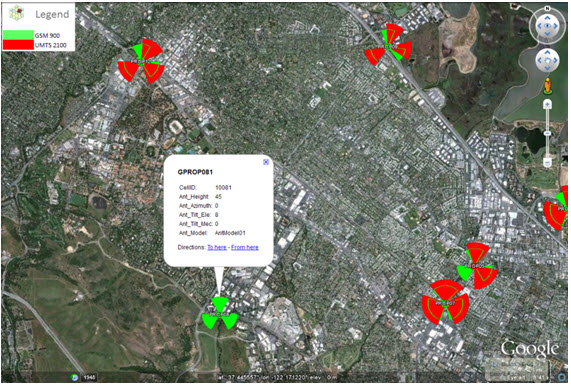
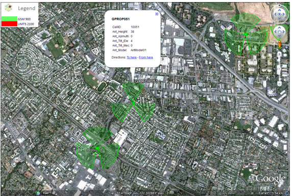
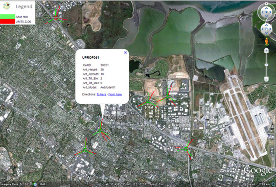
Now just one example plotting Network GSM 900, also with transparency. Another feature common to all: by clicking in the cell, we have the same information (in this case, we CellID, Height, Azimuth, Mechanical and Electrical Tilt and Antenna Model).

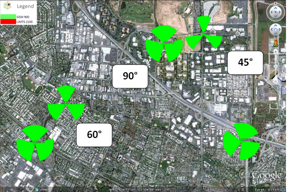
Another example of the GSM 900 network , but now with color without transparency. Also note that the horizontal opening of the antenna is also always obeyed.

An example with all networks (GSM 900 and UMTS 2100), only select lines instead of polygons to represent the cells. Note that all features remain, such as clicking in the cell to get information from it.

Well, we could continue plotting various combinations, but we were able to demonstrate what can be done, hope you enjoy.

Conclusion

We have seen how to create another customized application using Microsoft Access to plot Network Information in Google Earth KML / KMZ.

The comprehensive and functional, allows the practitioner to use on its network instantly, and also to make their own improvements / extensions.

Thank you for visiting and we hope that the information presented can serve as a starting point for your solutions and macros.

In particular, we thank the donators of telecomHall. We have already been sent the tutorial files to you, please check. If you have had a problem upon receipt, please inform.

We continue with the preparation of tutorials for various other modules, to be published gradually and in due course. At the moment, we have a series on Performance, with unique and interesting algorithms to ensure the best quality in your network.

Our search is continuing for the development of more simple applications, and allows us to improve our work, quickly and efficiently. Read all the tutorials and practice: the knowledge acquired can be your biggest difference!

Thank you.

Download

Download Source Code: Blog_027_HunterGENetwork(Application).zip (673.6 KB)