Introduction
When we talk about or KPI in Performance Analysis, what immediately comes to mind? While the answer to this question is particular to each person, we can think of a general answer in a report: a table, chart, map or even a combination of all.
No matter what the format of this report is, it is correct to state that it serves to tell us a comparison of indicators. This comparison may be on a fixed value, or on a different magnitude, among others. These are the ‘algorithms’ used.
But today we’ll see a previous step, althoug very important, and it is essential to generate any report - the use of base tables for data storage, and subsequent queries and analysis.
Purpose
From the data of counters (Excel, Text, etc…) import it into cumulative performance tables.
In other words, start creating the KPI Base Module, from where your tables will know quite a number of algorithms that assist in the analysis.
Note: do not confuse with what was presented at the Hunter KPI (Intro). On occasion, we learn how to import an excel file with data from counters to a database table. Today we go a bit further, where the raw counter data is imported, and accumulated in a repository (database tables). Anyway do not worry. Follow the tutorial and it will become clear in the end.
Our audience is from students to experienced professionals. Therefore we ask for a little understanding and tolerance if some some of the concepts presented today are too basic for you. Moreover, all the tutorials, codes and programs are at a continuous process of editing. This means that if we find any error, for example, grammar or spelling, try to fix it as soon as possible. We would also like to receive your feedback, informing us of errors or passages that were confusing and deserve to be rewritten.
File Structure
Again, there is no need to create another directory. We will work with the module Hunter KPI. We don’t need to create any new directory today because we are working with an existing module - KPI (1).
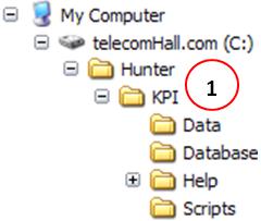
This structure and its files have been created in previous tutorial.
Base Tables
We understand as Base Tables those tables to accumulate performance data. The accumulation of data is accomplished through automated procedures that allow data to accumulate in standardized tables.
To get ahead a little on our side, and lose no time today to other issues such as creating tables, etc., consider that we have created three base tables.
Also, today we does not utilize the recommended practice that is to keep the tables in separate databases. We will do everything in that database (import files, create tables, queries, etc. …), because today we spend time in the learning process, and the fewer options to confuse our minds the better.
Boots and Settings
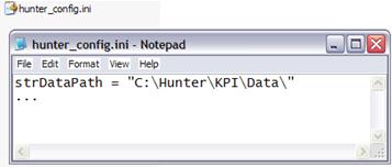
There are several ways to achieve the automatic processes. The simplest, but less indicated, is to write all the commands and settings directly in the code. It is the practice less used because whenever you have to change any data, such as the directory where your input data, you need to edit the code.
Other ways are through the loading of initial data from a file or table. In our modules we have chosen this second way: hauled almost all variables for auxiliary tables. Thus, for example to change the output or data directory, simply change the value in the auxiliary table.
Another advantage of this procedure is that we can have multiple functions and procedures in our code. And typed values directly in our code - it is called hard-coding - can have trouble changing everywhere. (Of course, we can use the Find -> Replace, but it already runs in our search for better solutions, and even if so, whether the instances are many, we spend time with here).
But only to not complicate, we also will not use it today - we again emphasize that we are concerned that you understand the process. Then it is easy to learn the improvements.
Homogenization
We already talked about this before, but it’s worth remembering the importance of standardization of data, ie, indicators that is common, regardless of what the technology or the provider of equipment. The easiest way to understand this is with the most standard of all indicators - traffic. That is, our table contains an indicator for traffic, be it GSM, UMTS or another.

Granularity of data, what for?
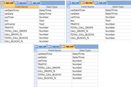
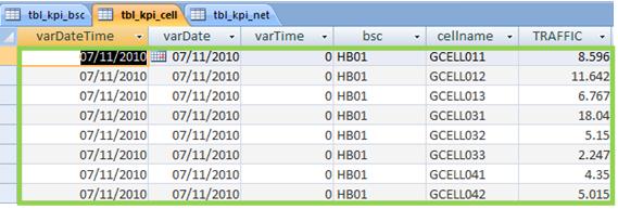
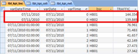
It’s also an important factor that we will see in the tables is cumulative it is interesting to accumulate data on all granularities. For example, we will have a cumulative table with key indicators at sector level (CELL), but we will also have a table with these same indicators grouped by BSC and/or RNC, and also by whole Network (NET). The figure below shows the design of three tables, with the three granularities shown (CELL, BSC and NET).
But why is that? Of course we can do queries on our main table, with the data of each sector. However, as the amount of data accumulated is growing, will also become more time consuming to run a query. Access has the power to deal with thousands and thousands of data at the same time, but if we have a report that uses the data in a more clustered, why not let them ready?
Frequency
The timing is also an item that we consider. Without going into further extend the theoretical concepts for today, we will work with a periodicity of 1 hour, ie for each group of counters, the value will represent the counts for exactly one hour. But this does not prevent data from being stored in other periodicity, for example, we have a table with the data accumulated in intervals of 1 day or even week. This will become more clear over time, now just know that our data were collected in the OSS - for this tutorial - with standard one-hour intervals.
Input Data
As you’re used to, before we start let’s define some dummy data to be used in our example today. Before, however, it is worth doing an observation on the input data.
It would be great if all the input data we use in our work all come in a standard format, whether Text or Excel, and these data were already in the format to import them. But this is not what happens.
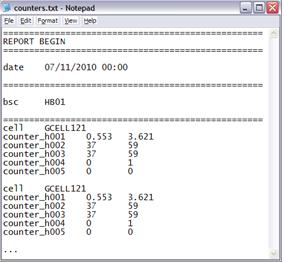
All data usually comes in a standard format, such as inserting a header with information for our case is undesirable. For example, an output format as shown below, with a header (1). We need to do a treatment before - delete the unwanted lines - before importing.
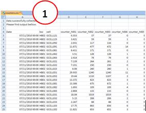
But our work can be even harder. The data source can be quite complex, depending on where we are getting our data. It is not uncommon to find input data in the format shown below, where they are being presented sequentially, ie, they need a larger treatment now, to put it in the desired format for import.
Hunter Tool is ready to import input data from formats above, and in several any new format that may arise. For this, we use a module that we will see shortly: Hunter Parser.
A parser is an application that takes data in a particular raw format, and transforms this data into a desired shape. Using the parser in the input data above, where they come from such commercial OSS, we input data in tabular format.
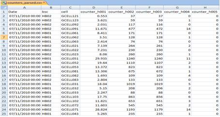
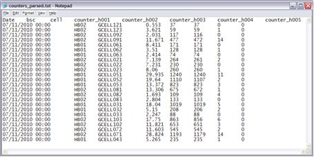
We will not concern ourselves with the parser for now, and we’ll assume that the data exported from our OSS are already in tabular format, and just import them. Note: As we speak, do not worry, soon we will be demonstrating how to perform this same procedure using the specific file format, not parsed.
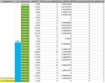
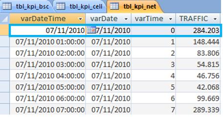
So continuing, we have a number of files exported, with the counters shown in the following counters:
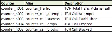
The periodicity of our data is hourly, so if the file is dated 07/11/2010 0:00:00 equal to mean that the data are collected from 00 to 01 hour of day 11/07/2010. That is, the data file has info for an hour.
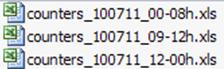
To demonstrate the automated process, we will assume that you have logged in OSS in some times and have downloaded the data. Let us assume that we then have three files:
-
counters_100711_00-08h.xls: with data from 0 to 8 am;
-
counters_100711_09-12h.xls: with data from 9 to 12 am;
-
counters_100711_12-00h.xls: with data from 12 am until the end of the day.
Note that if we add the 3 files then we will have one table with data from 24 hours. Not handy, we know how. But our goal is to learn how to make this process totally automated. So let’s continue.
But now a new problem arises: what if the files have duplicate data, will our data be replicated? In other words, suppose that for distraction, the first two files both have data from 8 to 9 hours of the morning.
Or better, if you’d append the data files into one, how would you do that? Probably you would open the first, paste data in it form the second and third, and save under a new name at the end, don’t you?
Well, know that the duplicate data would get there, and probably his report for example the sum of traffic of the day would be wrong!
There are forms of validation to expunge the repeated data in Excel for example we can apply a pivot table and get all the fields. In our procedure, importing the data into a database, let’s see how this kind of validation in a virtually transparent, that is, let’s not worry about it. We will use primary keys to do this job.
Primary Keys
When we talk about primary keys, of course means we get confused. This term is widely used by dba’s - or database administrators. Ok, deteriorated further.
Right, so simple, primary keys can be understood in our case as the set of fields that defines a record as unique. If we set the Date field from our table as the primary key, we would not have much success. Right away, the second record would have the same date, and the rule of the primary key - can not be duplicated - would error.
Much the same happens if we choose as the key to bsc primary. And if we choose cellname as primary key - to an hour data would be fine. But when we imported data from another hour (period), the cellname would repeat itself, and violate the rule of the primary key, resulting an error.
The solution then is to create a primary key so a table with several records for various days and times do not have duplicate records. And we do this by creating a composite primary key of all the fields that define a unique record.
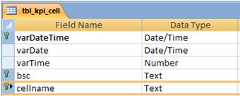
Sure, it was complicated, but we can not spell a lot about that today. Just accept that we must create a primary key with the datetime fields, and bsc cellname together, in the case of table tbl_kpi_cell.
Note: remember that in our Methodology of learning, we sometimes show something very quickly because we know that you will end up understanding when to use.
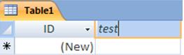
As a particular case, only to demonstrate, do the following. Create a table (Table1) with a field called ‘test’. No matter what type of field can be text itself.
Set this field as a primary key. To do this, go to Menu Design (1) of the table you created. Then select the field that you created (2) and click on Primary Key (3).
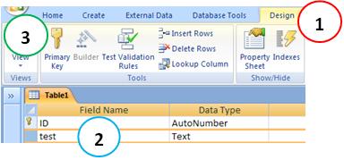
Note: Notice that Access automatically created a field in this table, the ID field of type autonumber, and has as a primary key - ignore this field and continue. We want the key as the field we created.
Now open this table, and enter a value. In the next field, enter the same value. Observe what happens.
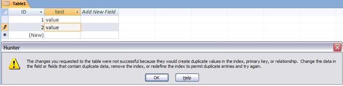
Access does not allow the field to be duplicated! To continue, press the ESC key.
Okay, that’s what we use as data validation, so you never have duplicate data in our tables.
To set the primary keys to ensure that our data will not be duplicated, click the fields with the CTRL key, then finally click the Primary Key.
We’ve talked enough for today, let’s now a little practice, on our real world.
How this module works
The goal today, as we talked about is learning the process of how the module works.
Simply put, we can represent the process through the steps below.
-
Download output files with OSS raw counters;
-
Save these files in the input folder (Data) of Hunter KPI module, so that they can be found and imported;
- Of course, this can be changed in future, where we can for example choose the module to import one or more files from a given folder. Today, we see the process in general terms, without many alternatives, only to not complicate the overall understanding.
- Import the file into a base table of counters;
- Here we have some more details that jumped today, as the parser or data processing that perhaps our input were not in the desired format. In the future we will see it too.
- From the base table counters, add (accumulate) on tables of performance.
- At this point we use the primary keys, we guarantee that we will not be repeated or duplicate data in our table, which would cause an error in our reports.
- Rename the file to import ading suffix ‘.imported’ and continue with the next file’s directory entry data.
- Continue this process until you run out the files to be imported.
Done. The data is already available in three tables:
- CELL : with data for each sector (without grouping).
- BSC : data grouped by BSC.
- NET : with pooled data across the network.
To run the process, we could have created an interface - we will also do this in the future. Today you must be tired of hearing, but we want you to ‘learn’ the process. If you do that, it will be fine. So to simplify, to run the process, just download the files from the OSS and place in the format as shown above (counters_parsed), and run the macro KPI_Main_RUN.
Note: Here is an interesting suggestion - duplicate some files, or enter into any a duplicate record. See what the end result - the accumulated data in tables - does not change, it is always correct, with no duplicate data!
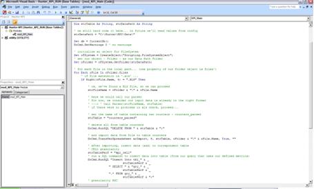
Code
Basically the entire automated process is accomplished through the VBA code. Let’s just highlight the new points.
The key is to use FileSystemObject . This option is one of the best for working with files and folders. Let’s talk quickly, we will use in other details.
The syntax to use is:
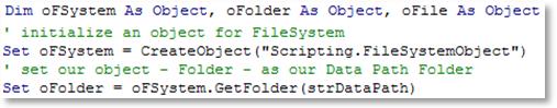
Once we loaded the our directory, we can make a loop on their properties. We use the properties files from the Folder object that we created from our directory entry and ready: we can perform the necessary actions (process each file, importing …)
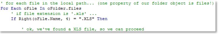
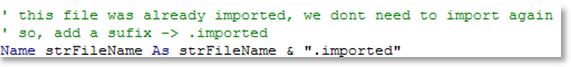
One of the interesting processes that we do is the following: Once the file is treated / imported, it need not and should not be imported and processed again. And how?
We use the Name command to rename files to a different extension of what we seek in the loop (if different from ‘. xls’). After each file is processed / imported, the file is renamed to “.imported”, and so the loop looking for files of type ‘.xls’ will not find this file (only the file of type ‘.imported’).
We have more news in the code for today. As always, we recommend you read, because it is fully commented.
References
These are the references that you should have in your project, to function as shown today.
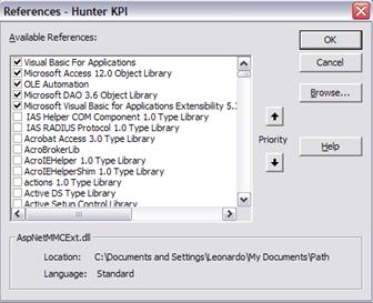
If any are missing, will appear as Away, and you should seek an alternative. In case of problems, please contact us. For example, instead of 12.0 may be that you have 11.0, if you are using Office 2003 instead of 2007.
Conclusion
We learned today the simplified automated import of one or more files with performance counters, and storing it in tables of performance.
This process involved several other concepts such as granularity (BSC, CELL, NET, etc …), intervals (hours, days, etc. …), pretreatment data (parser), performance tables with primary keys, performance metrics, etc… Besides some new concepts such as VBA FileSystemObject - used to work with directories and files, and the command Name - used to rename.
But it could not be all that was seen quickly, due to time limit, and also because we can not learn everything at once. But do not worry, we will speak of these matters, as we evolve, and all catch up. Anyway, note that we are increasingly learning new things, and very soon we will be using the tools in a completely professional.
Our search is continuing for the development of applications more simple, and allows us to improve our work, quickly and efficiently. Read all the tutorials, keep practicing and acquiring knowledge - this is your greatest differential!
We hope you’ve enjoyed. If you have any doubts, find the answers posting your comments in the blog or via our support via chat or email.
Till our next meeting, and remember: Your success is our success!
Download
Download Source Code: Blog_018_Hunter_KPI_(Base_Tables).zip (71.2 KB)