Introduction
The KPI is a major part in any cellular network. And the same skills to analyze, therefore, a major task for us who work in this area. So, let’s see a little of both today: more theoretical knowledge that we will use from now on in several modules that work with KPI Hunter, and a little Access database, specifically to learn to work with data in tables and queries.
Purpose
Begin practicing the concepts of the analysis of the cellular network through statistical counters manipulating data in tables and queries.
Our audience is from students to experienced professionals. Therefore we ask for a little understanding and tolerance if some some of the concepts presented today are too basic for you. Moreover, all the tutorials, codes and programs are at a continuous process of editing. This means that if we find any error, for example, grammar or spelling, try to fix it as soon as possible. We would also like to receive your feedback, informing us of errors or passages that were confusing and deserve to be rewritten.
File Structure
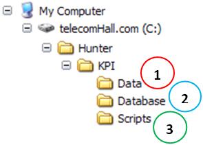
Today we will not create any new directory, as it has already been created in previous tutorial. The new files should be stored following the Hunter methodology, ie, files with the raw data in the Data directory (1) and databases in the Database directory (2). In the Scripts directory (3), as its name suggests, we have the codes we use in the module.
More details will be informed as we evolve.
What’s the worst sector of the network now?
Answer honestly: Do you know how to analyze performance data from a network?
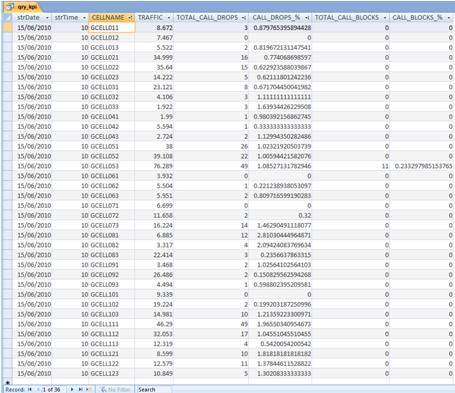
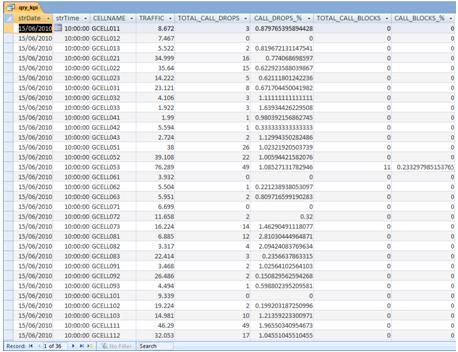
In other words, if someone gives you a basic table as shown below with data from a certain time, and at least the basic indicators - traffic, drops, blocking - can you say what the is worst sector of the network at that moment?
Well, most people will say yes. And really, it is not so difficult: for example, using the facility to sort in ascending or descending, you’ve achieved something. Okay, okay, but what indicator will you use?
We go a little deeper… Assume that you will use the indicator drops to define what the worst sector. Will you use the absolute number(TOTAL_CALL_DROPS) or percentage (CALL_DROPS_ %)?
To show that it is not as simple as it seems, let’s see examples …
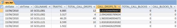
If you choose the percentage indicator (CALL_DROPS_%), and sort in descending order (from highest to lowest), you will say that the worst sector of the network is the GCELL081 - that showed a rate of dropped calls of 2.8%.
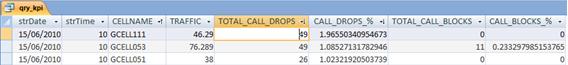
But if you instead choose the absolute indicator (TOTAL_CALL_DROPS), and also sort in descending order, will say that the worst sector of the network are actually two (there was a tie ) - are the sectors GCELL053 and GCELL111, both with 49 falls during the period.
And then, what is the worst: GCELL081, GCELL053 or GCELL111?
The answer to this question depends on several factors, such as those sites which cover the principal’s office of our company! Jokes aside, the prioritization based on the importance of the site should always be taken into account, as other factors that we will see with time.
Anyway, one way we can use to define what is the worst sector of the network at the moment is to use other indicators together.
Shall we continue in our example, choose another indicator (in this case, the blocks) and sort descending.
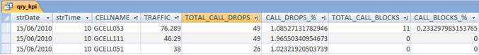
See it now becomes easier, especially in our particular case, where the sector GCELL053 was the only that has blockage (absolute, and consequently also percentage).
Not taking into account other non-technical factors, we can then answer that the sector that requires immediate intervention is the GCELL053.
Realize that in a real network, the number of sectors is much greater. And also in the practical world, there are used more indicators - although as we discussed, the basic indicators almost always define the problems and the others are used more as an aid to problem solving.
Ok, we already identified the worst sector, and now, what to do?
To find the worst sectors - or offenders as we refer from now - it’s fairly simple. But it is only the beginning of our work …
An efficient analysis of performance must necessarily take into account several other reports, such as the alarm report. Ie, that sector is worse with a problem, for example hardware.
Or depending on the presenting problem, is there any action that will solve the problem - such as an expansion or even adding a new site?.
Based on this information we will take appropriate action. And of course, all depending on our area of expertise, such as O&M, Planning or Optimization.
If our area for example is the Optimization, the indicator that matter most in this case the suit will be dropped calls. If we act in network Planning, let us worry about the traffic growth and blockages. And if we work with for example the Maintenance and Operation, probably will use a much better indicator of failure - although in future we will see how to identify deficiencies in the maintenance and operation of network using only the indicators shown above!
We’ve talked a lot about what to do. Now let’s learn a bit more about tables and queries in the database, and how to use them to analyze the data.
Access Tables
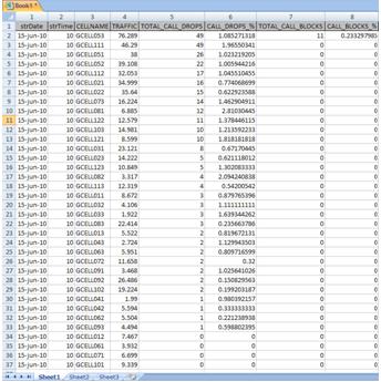
We’ve talked about tables in the first tutorial, especially in the tutorial Hunter Network, but let’s remember. Tables are sets of records, but it’s easier to imagine a table reminiscent of data in an Excel worksheet. The data that we used above could be quietly in an Excel worksheet as shown below.
Yes, we can work with data in Excel! But there are some advantages to learning to work with the database. In this case, we will work with one of the simplest database that exists, which is Access - also from Microsoft, such as Excel. This means that if you already use Excel, you will learn more easily using Access, not least because many commands are common Office Software. See for example how is our Excel worksheet after being “imported” into the database.
One advantage is the ability that Access has to work with more data than Excel. Although the newest version of Office (2007 or 2010) has improved considerably the limitations of Excel in terms of data capacity, Access continues to be much better for this purpose.
Okay, still can not understand why Access is better…
Another advantage is the ease we have to create SQL queries to access data.
If you do not already know, SQL is a language for access data in a database. It is both simple and powerful. Its syntax is very intuitive. For example, see an SQL statement: SELECT * FROM mytable;. This is a very simple SQL statement, and it means more or less: Select all data from the table MyTable.
Creating queries in Access is simple, and has also been shown in the first tutorials. Anyway, as we are giving examples, let’s create a query.
But first, let’s go back to recall a concept already present: the concept of linked tables. We could create this and other queries within the same database where is the table of our example. However, as we has already learned in the first tutorial, it is better to separate the part thath accumulate dat from the part of queries. This has shown for several reasons, one is that it is easier to separate the backups.
So, let’s assume we have a table available with the data from the previous tutorial, in the database Hunter_KPI_DB.mdb, located in the Database folder of KPI module.
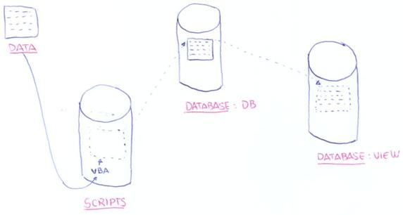
We create a new blank Access Database with the name Hunter_KPI_View.mdb, also located in the Database folder. This database will be used as a data viewer (VIEW) for data we have in our repository (DB).
Remembering always: even if it seems a bit complicated, it is not! When you start practicing, you’ll realize that. The figure below tries to explain a bit as is the case, but even if you still do not understand, continue.
Ok. Let’s first create a query in the database qry_KPI (VIEW).
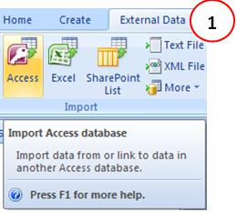
But this database is empty, there is not even a single table. So we will first link the table - we’ve seen another tutorial on how to do it too. But let’s go again, and access Menu from Access External Data (1).
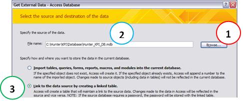
Then click the browse button (1), and select the database Hunter_KPI_DB.mdb (2), which is our data repository. Select the option to link the table (3), and click the OK button of this dialog box.
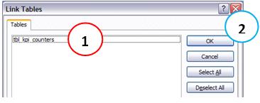
It brings up a dialog box that you. It allows you to choose which tables in the database repository will be linked in this new empty database. That is, tables that you will have access to data, but the data itself is stored physically on the other bank - so we say that database visualization is lighter. Then Mark the (only) available tbl_kpi_counters table (1), with our dummy data, and click the OK button (2). Done - our table was linked successfully.
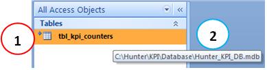
Note that the table becomes available. Can you identify that it is a linked table by the little arrow beside it has (1), and when you put the mouse over, it shows that the database from where is the physical table (2).
Phew, have not begun yet, and already gave to tire … But it’s good because we are remembering and learning. Always remember that the goal is that you learn all that is fully shown.
Now on to create the query
To create a query, remember that there are several ways, one is through the Create Menu (1) -> Query Design (2).
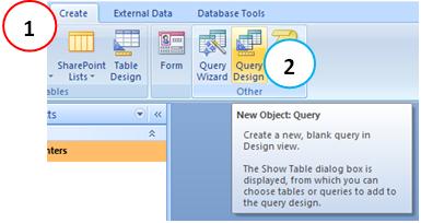
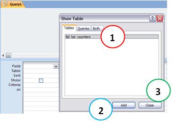
The interface structure of Access queries is very friendly and very helpful in building the SQL. So we create a new query, he asks us what are the tables and/or queries that we use. (That’s right, we can do queries on queries, but let’s talk about it later, not to lose the focus right now). To start the issue of queries using the interface, select the table you want to access the data from - tbl_kpi_counters - and click the Add button (2). As we only use this table, also click the Close button (3).
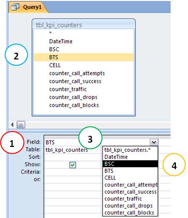
This is the editing interface. Query fields (1) can be directly the table fields or calculated fields. We will use both. And to show the query field of a table, you can click on any field (2) and drag it to a blank column of the query (3), or choose from the list box (4). This is quite superficial, all the details and possibilities you learn by practicing.
And a calculated field is defined by a field name following the “:” and the expression. Again remember we talked about it in the first tutorial, and we are reviewing soon. If you have any questions, please read the first tutorial, or else contact support.
Calculated fields can be results in math, or expressions, among others. The universe is big. For example, in our query, we want to separate the date - which contains the date format date / time field with a date only, and a field with time only. We can have everything: a field with date and time, another with date and another with only the time. You decide which fields you want in your query.
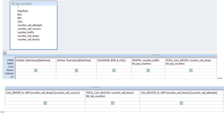
The function to extract date is the DateValue (), so we have the calculated field strDate: DateValue ([DateTime]). Likewise, the function to extract the Access Time is the TimeValue (), and we have the calculated field strTime: TimeValue ([DateTime]). Over time, we will learn numerous other features that will help us enough in the manipulation of data using queries, do not worry you’ll learn each one as you need to.
The mathematical calculations are done using the common signs of operation. To multiply, use ‘*’, and to divide, we use ‘/’.
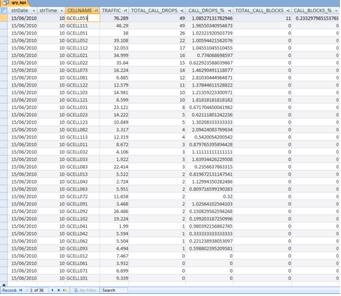
See then how does our final query qry_KPI in a common format for presentation. (The image was divided into two, just for better viewing).
The result of this query, you can see through Menu Design (1) -> Run (2).
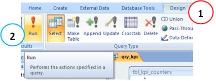
Note: You may have noticed that the tip that appears when the mouse is over the button to click Run reports that he will perform the action specified in the query. Why is that? Well, actually let’s talk about it later, and has also talked in the first tutorials. SQL queries may have other purposes than just selecting data, as is the standard and is what we are looking to start learning.
There are options for SQL to create a new table from the data specified in the instruction to add data (accumulate) in other existing tables, among other much more advanced. We will use quite all the options, but first we need to learn the basics, or select queries. In the next tutorial KPI for example you will learn how to use queries to create tables and accumulate data to create our system.
Returning to our point, after clicking the run, we have the query result.
Gee, and we both walked to a simple table?
Calm down, it was just to show how to create and use a query. This query was saved with the name qry_KPI, and when executed, displays the data in the table are those which tbl_kpi_counters.
But in our example, the data is only one period, and few sectors. And what about if we have a lot of accumulated data?
Other query options
At the risk of being being a bit repetitive - as these queries concepts were seen in the first tutorials - let’s illustrate some uses of filters, conditions, expressions, etc… in queries.
The SQL Query has several options beyond simple Select, which means select. Besides the replacement options as per instructions of the Select Update - updating data from a table instead of selecting, as have several other ORDER BY ordering data.
One of these options, or we may call the arguments of SQL, is the WHERE clause, ie one or more conditions to be obeyed.
Oh oh … returned to complicate … Sure, we have listed.
See the instruction that we speak up, but now with a conditional clause: Select * from MyTable Where Name like ‘telecomhall’; Now, this statement means something like this: Select everything from table mytable whose Name field has the value telecomhall!
In the Access interface, the conditions are inserted in line criteria. For example, if in our query qry_kpi_counters we insert the criteria Like “* CELL08 *”, what does it means?
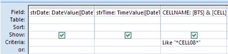
Okay, we were not fine. You may not even know that we can also use wildcards in expressions of text. What is this? Well, wildcards work more or less as a mask to accept any data type. For example, if you use the ‘*’ means that it accepts anything. In this case, we want the field to be as CELL08, ie we want to select all data from the query whose cellname field has the value text with anything, followed by CELL08 in turn followed by anything! It’s getting kind of abstract or crazy? Relax, it’s because you have not practiced …
Running the query with this criterion, we have the following result.
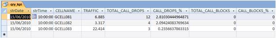
Nor has much practical sense, but served to show how to use criteria as well as wildcards.
And what happens if we specify a condition that does not exists in the table? Simple, the query returns nothing. Below is the query output with criterion #10:00:00#, ie a time that we know exists, and exit #11:00:00#, a time - that is a condition- that doesn’t exists in our data.
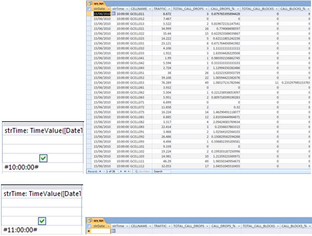
Note: If you are aware, has noticed another identifier, the symbol #. This symbol is used to inform that the value we are using is a date or time.
An option that is also very important and useful in SQL is the GROUP BY clause, or grouping. It is important because it allows the use of various group functions as sum, count, etc… However, it is an option that many people have difficulty understanding, but with no reason.
We use the grouping option when we want a result - of course - grouped into one or more fields. What happens is that people often use the group clause, but they forget that they need to arrange the fields so that it is possible that grouping.
For example, if you want to count how many sectors we have in our query, what would you do? Sure would use the group clause.
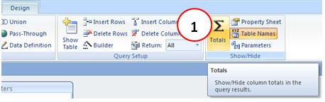
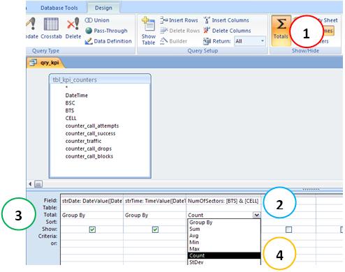
Okay, in the editing interface of the Access query, specify that you want this query to group data by clicking the button Totals (1).
But that alone? No, that’s the thing. The query will group all records the same, but so what? To work, and for example we have a query that returns in the amount of records, we have only the fields that will be grouped.
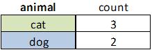
Alright, alright … is confused. Let’s see a more graphical and intuitive. Suppose a simple table with animal and name.
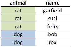
Now suppose you want to count how many animals are in each, ie counting the records of the animal (field animals) grouping field name. If we’re using a SQL query, and you simply insert the clause group, the result is as shown below.
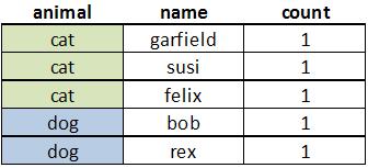
Realize that you need to delete, or in other words, it can also display this field in the query, but falls in the case shown above. So, if you group only by the correct fields, you can then obtain the expected result.
Maybe it has not yet been entirely clear, but we hope you understand at least the following for now: you must choose the appropriate fields according to the result you need.
In the case of our query, we will use the group clause and amend our query so that the result is the count of sectors for the day and time available. To do this, click the button Total (1), erase the other fields that are not Date, Time and cellname (2), and changed the Collate option for the total lines (3) Field cellname to count (4). Just to be more intuitive to change the name cellname NumOfSectors.
By running the query, we find the results like expected.
We would still have plenty to show, query options, among others. However, for today is enough that you have learned some concepts, or rather, set what we have learned before, and seen as the data handling can be done with Access.
But ultimately, what’s interesting about all this?
Sure, there’s nothing practical in what we saw. But that was intentional. We’re here teaching, and everything we need to be well understood by you. One reason is that because we use more and more queries, and these in turn increasingly becomes more and more complex.
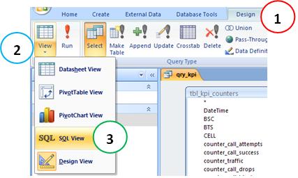
One thing that we didn’t speak, and it is important is this: every time you are editing a query in the Access interface, you can quickly check what is the SQL syntax of the same ! Simply access the Menu Design (1) -> View (2) -> SQL View (3).
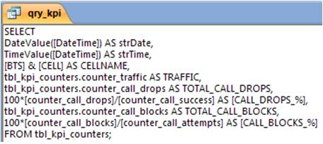
See the SQL syntax of our original query qry_KPI. And the coolest of all, you can edit the query using the interface much, much typing in the actual SQL! That is, if you are great using SQL, you can simply type in your commands and execute them. Particularly, we prefer to use the Access interface, and if necessary, make adjustments via SQL in SQL View.
Note: there are certain types of queries - and forward - that have no graphical representation, through the Access interface - or any other program, such as UNION queries. At the right moment, we will use every type of advanced query and explain everything in detail. You’ll be amazed at how SQL queries are really powerful.
An interesting use of the SQL View is a possibility that we have to edit the SQL, for example, in Notepad or even creating syntax through concatenated fields in Excel.
Another more important thing about tables and queries is that they can all be accessed via VBA code! In fact, they can even be created via VBA!
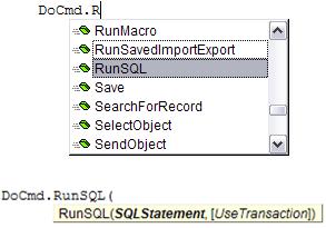
Through command Docmd.RunSQL (SQLStatement) can run pretty much everything we need.
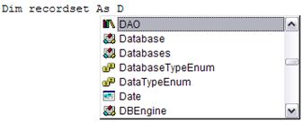
And data from tables and queries can also be accessed through RecordSets, another powerful feature of the databases. RecordSets can be understood as a recordset in memory, and we’ve talked about this in a previous tutorial - in fact, already used RecordSet in some modules such as generating the network data in Google Earth (Hunter GE Network).
Handling objects using the Access database, either through its interface, either through VBA code, and we can create amazingly powerful applications, and meeting all these applications result in an integrated system, the Hunter.
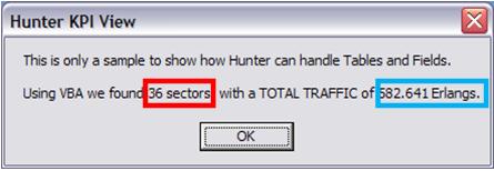
Just to finish, we create a module with VBA code that does some simple manipulations with qry_KPI query data, and returns as a result the total number of sectors and the sum of traffic in a simple dialog box. Of course, in our future reports will be so much better than a message box, but it serves to demonstrate our purpose today.

Do not worry, this code is commented by more than normal - since it is a sample code. Anyway, if in doubt, contact support.
We also create a macro - qry_KPI_VBA_RUN, as already explained in other tutorials, just to run the code created in the module.
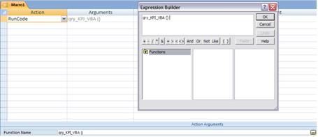
So, very easily, run this macro and you will see the result instantly.
Well, that’s it for today. Although a good start, we still have much to learn. But we believe that is enough for today. If you can understand and practice what has been presented, will be prepared to accompany the upcoming modules. As you already noticed, all the codes provided are commented, and is very easy to read and understand what is being done.
Conclusion
Today we had the opportunity to recall some concepts, and learn some new ones used in the manipulation of tables and queries in Access database. In terms of performance analysis, although we saw very little that can be used in practice, but we had an overview of the possibilities we have, or what we construct. The reason is simple: we are more concerned with what you learn, and it can not perform any analysis of how well made the concepts seen here are not fully understood.
The end result, although simple, already enable us to see that we can create extremely powerful tools, but simply and efficiently, just by will and creativity. This is the vision we have the Hunter system, and you should now be starting to see how it is incredibly amazing, aren’t you?
We hope you’ve enjoyed. If you have any doubts, find the answers posting your comments in the blog or via our support via chat or email.
Till our next meeting, and remember: Your success is our success!
Download
Download Source Code: Blog_015_Hunter_KPI.zip (88.0 KB)